Differential Impact Detection
Learn how Statsig automatically flags experiments with extreme differential impacts on sub-populations.
What is Differential Impact Detection?
Experiments can have interesting effects on sub-populations that are easily missed. They might have a bug that impacts only a certain browser, OS, or country. If the topline impact isn't significant or is canceled out by other changes - these are missed.
Statsig will automatically flag experiments when extreme differential impacts are detected for any sub-population you have configured. Once configured, experiments are analyzed for differential impact when Pulse is loaded after Day 1, Day 3 and when the Target Duration is met.
Enabling this
Configure the "Segments of Interest" you want automatically evaluated for Differential Impact Detection. On Statsig Cloud, these are user properties in the User Object you configure when using the Statsig SDK. On Statsig Warehouse Native they can be configured as an Entity Property too.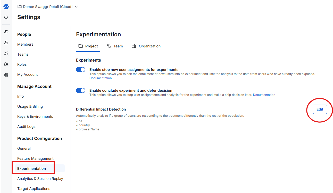
This feature is also referred to as Heterogeneous Treatment Effect or Segments of Interest.
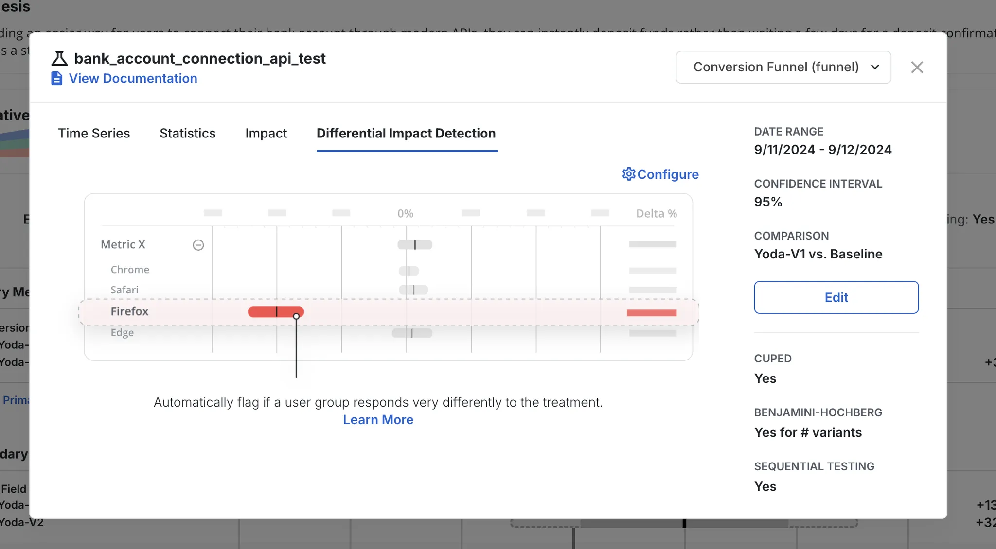
Seeing Differential Impacts
If extreme outliers are found for a segment you have configured, Statsig will flag this when you're looking at Pulse results. You will be able to see the data broken out by segments in the Explore section of your Pulse results.
Methodology
We use a Welch’s t-test to compare the treatment effect for a particular segment of users to the treatment effect for all other users since we expect to potentially see unequal population variances when comparing user segments.
The average treatment effect is calculated as follows:
The variance in treatment effect is calculated as follows:
The n of the treatment effect is calculated as follows:
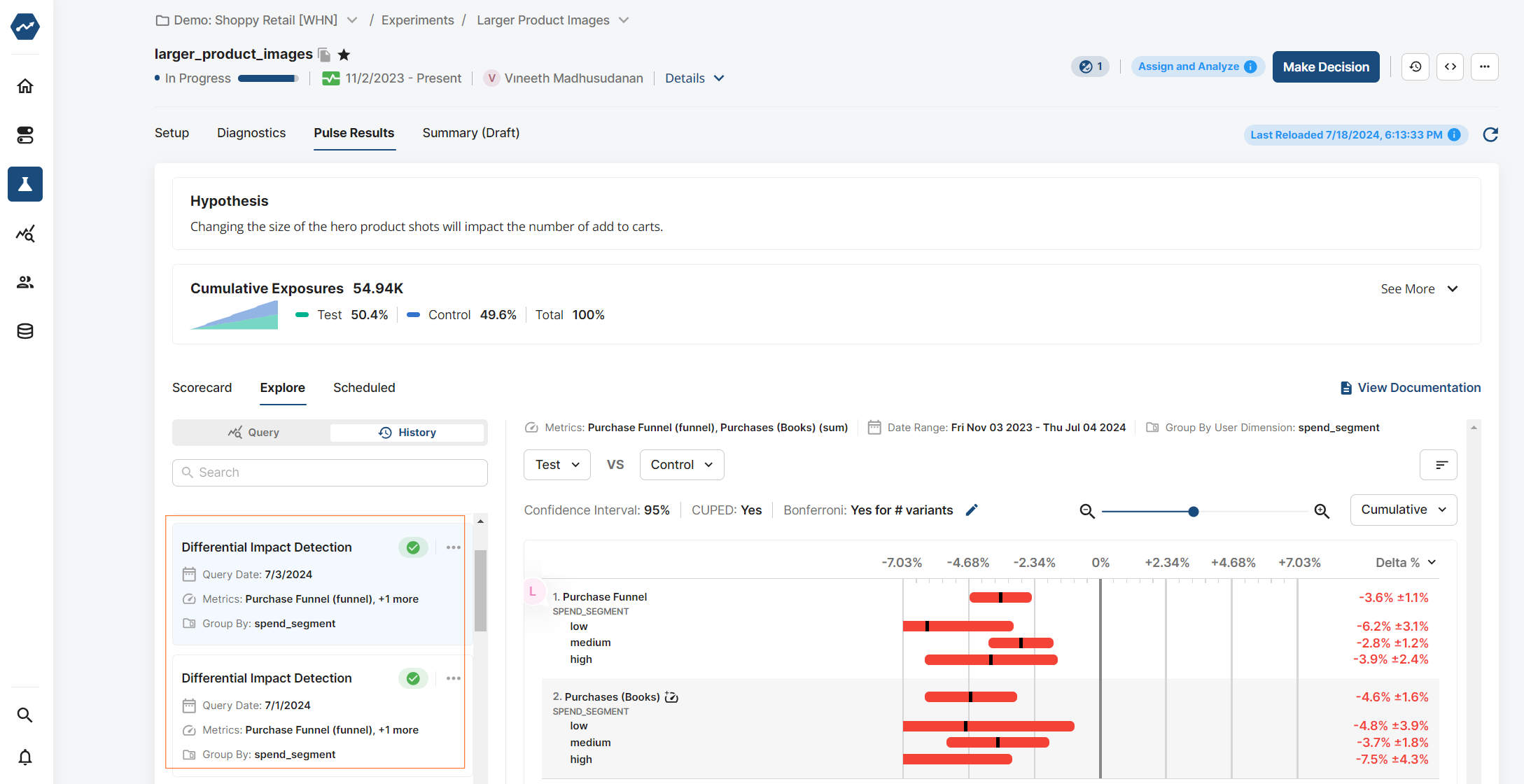
Viewing Results
You can go to the explore tab of your experiment and filter to the Differential Impact Detection query type to see all historical analyses.
Was this helpful?