Geotesting Methodology

How geotesting differs from standard A/B testing

Standard A/B testing relies on a few core assumptions:

1. You can reliably and randomly split your users into similar groups.
2. While each group has heterogeneity inside it, random user-level variations average out at larger sample sizes, resulting in homologous (similar) groups.
3. You control how each group gets treated, and there's no interference between groups.

When these core assumptions are true, the treatment effect is the only observable difference between the groups. Measure each group’s mean value and find the difference between them.

There are times however when these assumptions don’t hold:

• Your intended treatment can’t be controlled and scoped to the user level
• You don’t know who the users are
• You can’t track outcomes at the user level

Running geographically-based campaigns is a prime example that often features at least some of these violations. Examples include:

• Some classic marketing, like billboards, can’t be randomly split between test and control users at a given location. You can’t track who sees them and how they act afterwards.
• Some digital campaigns might be able to split users 50/50 (if the platform allows it), but without user-level data that can be tied to outcomes of interest, you can’t determine how the two groups performed.

Using synthetic controls

“Geotesting” as referred to here is an experimental framework that relies on a different basic setup than AB tests:

1. Split your users into geographical boundaries at some useful level (zip codes, states, countries, etc.).
2. Apply a known treatment in some “treatment” geos, and no treatment in some “control” geos.
3. Use the control geos to figure out what would have happened in the treatment geos had no treatment been applied (that is, “synthetic” results).
4. Measure the delta in the treatment geos between the actual and synthetic values.

Determining what would have happened is the most difficult part of this setup. Deducing things that didn't occur is generally unreliable, but in some circumstances there is enough predictability in a system to make it possible.

Geotesting relies on sufficient correlations between control and test geos to make predicting this “counterfactual” possible. General trends and seasonality tend to be shared across some geos.

Example: pretty much all zip codes in the United States exhibit similar quantities of mail sent on any given day. If you were to split zip codes 50/50, you could reasonably infer that the two groups would see similar trends.

Estimation approach

There are many ways to estimate unknown data from other known data, depending on a multitude of factors. In the case of Geotesting, the data has:

• timeseries data that is autocorrelated (i.e. data is correlated from one day to the next within a group)
• timeseries data that is correlated between groups
• regular seasonal patterns that repeat at regular intervals
• granular data from among many distinct geographies

Plotting a metric of interest for a set of relevant geographies can show these relationships clearly.

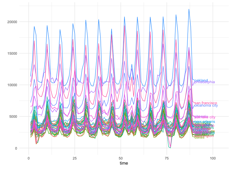
Example data from the GeoLift package walkthrough.

But what happens when a campaign runs in only some of these geos? How can you tell if a fluctuation in this graph is random noise or a statistically significant result?

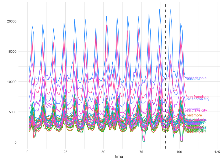
A marketing campaign that starts on day 91 (black dotted line) could have affected the treatment cities of Chicago and Portland. But how do you distinguish any real effect from all the noise?

Causal inference modeling addresses this question. A variety of models and methods have been developed for this purpose. The basic steps are:

• Split your geos into test and control groups.
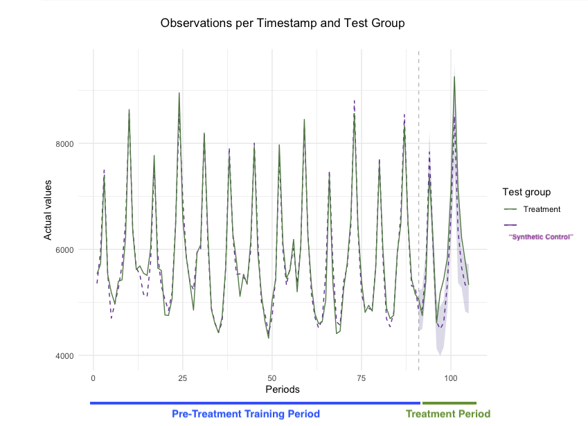
• Using the pre-treatment period data, train a model on the control data to predict how the treatment geos behave.
• Using the post-treatment period data for the control geos, create a “synthetic control” dataset to predict how the treatment geos would have behaved after the treatment event.
• Subtract the synthetic data from the actual observed data to determine the induced effects of your treatment on the treatment geos.

When your training data is able to produce strong models that can predict metric outcome well, you end up with strong estimates of an induced effect:

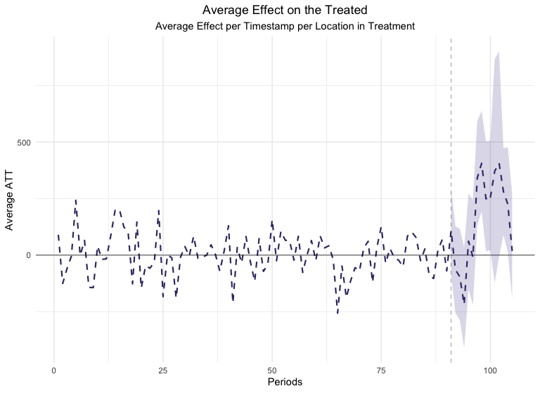
Subtracting the modeled Synthetic Control values from the observed Treatment values reveals any incremental effect for the Treatment geos.