Data Best Practices
Best Practices for using Statsig in your warehouse
Cost management
Statsig's pipelines use many SQL best practices to reduce cost, and smaller customers can run month-long analyses for a few cents.
Following these best practices helps keep costs under control and consistent.
Go to Compute Cost Transparency to understand how much compute time your experiments use.Follow SQL best practices
Statsig uses your SQL to connect to your source data. Common SQL issues include:
Avoid using
SELECT *, and only select the columns you needSELECT *leads to a lack of clarity in what you're pulling/require for other users- For warehouse like Bigquery and Snowflake, it can increase the scan/size of materialized assets like CTEs in snowflake
- This leads to higher query runtime and higher warehouse bills
Filter to the data you need in your base query
- This reduces the scan and amount of data required in future operations
- You can use Statsig Macros (below) to dynamically prune date partitions in subqueries
Group common metric groups into a single Metric Source
- Statsig filters your source to the minimal set of data and then creates materializations of experiment-tagged data. To maximize the effectiveness of this strategy, have metric sources that cover common suites of metrics you usually pull together.
Cluster/Partition tables to reduce query scope
- Most warehouses offer some form of partitioning or indexing along frequently filtered keys. In warehouses with clustering, the recommended strategy is:
- Partition/Cluster Assignment Source tables by date, and then your experiment_id column so you can scope experiment-level queries to that experiment
- Partition/Cluster Metric Source tables based on date, and then the fields you expect to use for filters
- Most warehouses offer some form of partitioning or indexing along frequently filtered keys. In warehouses with clustering, the recommended strategy is:
These best practices are generally true across all warehouses, especially as the datasets you use for experimentation scale.
Materialize tables/views
Since Statsig offers a flexible and robust metric creation flow, it's common to write joins or other complex queries in a metric source. As tables and experimental velocity scale, these joins can become expensive because they run across every experiment analysis.
To reduce the impact of this, best practice is to:
- Materialize the results of the join and reference that in Statsig, so you only have to compute the join once
- Use Statsig macros to make sure partitions are pruned before the join, and you only join the data you need
Use incremental reloads
Statsig offers both Full and Incremental reloads. Incremental reloads process only new data and can be significantly cheaper on long-running experiments. Advanced settings in the Pulse advanced settings section (also available as org-level defaults) help you make tradeoffs to reduce total compute cost. For example, the "Only calculate the latest day of experiment results" setting skips timeseries. This setting can run large full reloads (for example, one year on 100M users) in 5 minutes on a Large Snowflake cluster.
Reload data ad hoc
Depending on your warehouse and data size, Statsig Pulse results can appear in as little as 45 seconds. Because pipelines have flat costs, reloading 5 days isn't 5 times as expensive as loading one day.
If cost is a concern, choosing which results to schedule versus load on-demand can significantly reduce the amount of processing your warehouse has to do.
Use Statsig's advanced options
By default, Statsig runs a thorough analysis including historical timeseries and context on your results.
Use metric-level reloads
Statsig offers Metric-level reloads; this allows you to add a new metric to an experiment and get its entire history, or restate a single metric after its definition has changed. This is cheaper than a full reload for experiments with many metrics, and is an easy way to check guardrails or analyze follow-up questions post-hoc.
Use Statsig's macros
In Metric and Assignment sources, you can use Statsig Macros to directly inject a DATE() type that is relative to the experiment period being loaded.
{statsig_start_date}{statsig_end_date}
For example, in an incremental reload from 2023-09-01 to 2023-09-03, this query:
SELECT
    user_id,
    event,
    ts,
    dt
FROM log_table
WHERE dt BETWEEN {statsig_start_date} AND {statsig_end_date}
resolves to
SELECT
    user_id,
    event,
    ts,
    dt
FROM log_table
WHERE dt BETWEEN DATE('2023-09-01') AND DATE('2023-09-03')
This is a powerful tool since you can inject filters into queries with joins or CTEs and be confident that the initial scan is pruned.
Avoid contention
Resource contention is a common problem for Data Engineering teams. Large runs in the morning to calculate the previous day's data or reload tables are typical. On warehouses with flat resources or scaling limits, Pulse queries can be significantly slower during these windows, and can also slow down core business logic pipelines.
The best practice is to assign a scoped resource to Statsig's service user. This has a few advantages:
- Costs are easy to understand, because anything billed to that resource is attributable to Statsig.
- You can control the maximum spend by controlling the size of the resource, and independently scale the resource as your experimentation velocity increases.
- Statsig jobs don't affect your production jobs, and vice versa.
If this isn't possible:
- Schedule your Statsig runs after your main runs (this also ensures the data in your experiment analysis is fresh).
- Use API triggers to launch Statsig analyses after the main run is finished.
Analytics optimization
When using Statsig’s Metric Explorer to visualize data in your warehouse, optimizing table layout and clustering configurations can greatly improve latency. This section describes best practices you can use to improve the performance of analytics queries, with recommendations for some of the most commonly used warehouses.
BigQuery
Table layout: partitioning and clustering
Partition on event date and cluster on event when defining your events table. This improves performance because most queries filter for the event name and the time it was logged. When defining the partition on event date, truncate the timestamp to day-level granularity instead of using the raw timestamp (which would otherwise have millisecond precision, resulting in very high cardinality).
-- Create an events table partitioned by date and clustered by event.
CREATE TABLE dataset.events (
  ts TIMESTAMP NOT NULL,
  event STRING NOT NULL,
  ...
)
PARTITION BY DATE(ts)
CLUSTER BY event;
BigQuery's support for applying a cluster to an existing table is limited. Adding a cluster to an existing table doesn't automatically recluster the data immediately. If you need to repartition on event date or add a cluster by event, create a new table with the correct partitions and clusters using your current table.
-- Using an existing events table, create a new table that is partitioned by date and clustered by event.
CREATE OR REPLACE TABLE dataset.events_new
PARTITION BY DATE(ts)
CLUSTER BY event
AS
SELECT *
FROM dataset.events;

-- (Optional) Swap the name of your new table with the old one for consistency.
DROP TABLE dataset.events;
ALTER TABLE dataset.events_new RENAME TO events;
Databricks
(Preferred) Use liquid clustering
When making clustering decisions in your events table layout, liquid clustering provides a flexible approach that allows you to modify your clustering keys without needing to manually rewrite existing data.Use liquid clustering for your events table as follows:
-- Enable liquid clustering for your events table.
ALTER TABLE events SET TBLPROPERTIES ('delta.liquidClustering.enabled' = 'true');

-- Cluster on the event column.
ALTER TABLE events ALTER CLUSTER BY (event);

-- Trigger clustering using the OPTIMIZE command.
OPTIMIZE events;
If you frequently update your events table, Databricks recommends scheduling OPTIMIZE jobs every 1-2 hours. This incrementally applies liquid clustering to your table.
(Alternative) Partitioning and ZORDER
If you choose not to use liquid clustering, partition on a single low-cardinality column such as the event date. Avoid adding more than one column on the partition unless necessary, and don't partition on a column with cardinality exceeding one thousand. Use a generated column to simplify pruning:
-- Define a partition on the event date generated column.
CREATE TABLE events (ts TIMESTAMP, event STRING, event_date DATE GENERATED ALWAYS AS (CAST(ts AS DATE))) USING DELTA PARTITIONED BY (event_date);
Use ZORDER to colocate similar values within a file for a high-cardinality column, which improves query performance through data skipping. Apply this to the event column:
-- ZORDER by the event column to improve data skipping.
OPTIMIZE events ZORDER BY (event);
Use a scheduled job that runs OPTIMIZE on the last week's event data to improve query performance by compacting small data files into fewer, larger files:
-- Periodically optimize the events table based on the last week of data.
OPTIMIZE events WHERE event_date >= current_date() - INTERVAL 7 DAYS;
Avoid partitioning on a combination of event date and event. Even for small queries, this combination creates significant overhead: with 500 events, a 30-day query hits 15,000 partitions. Instead, partition only by date and use ZORDER on the event.
For extra parallelism without introducing too many partitions, ZORDER by an additional bucket column, defined as follows:
-- Add bucket column for extra parallelism.
ALTER TABLE events ADD COLUMN event_bucket INT GENERATED ALWAYS AS (pmod(hash(event), 16));

-- Rewrite data into new files based on this ZORDER key.
OPTIMIZE events ZORDER BY (event_bucket);
Partition pruning
Dynamic File Pruning enables Spark to prune partitions based on filter values at runtime. Enable it if possible using:
-- Turn on Dynamic File Pruning.
SET spark.databricks.optimizer.dynamicFilePruning = true;
Handling skew and joins
To rebalance skew and adjust join strategy, turn on Adaptive Query Execution:
-- Turn on Adapative Query Execution
SET spark.sql.adaptive.enabled = true;
Compute choices
The Photon query engine allows faster query execution with more efficient use of CPU and memory. If possible, enable it for your compute cluster or SQL warehouse.
Redshift
Table design: distribution style and sort key
Because Redshift doesn't support partitioning by column, use a sort key instead. Most event tables are append-only and time-based, so use a compound sort key on (timestamp, event) to order data by time. Because all analytics queries filter on timestamp, this allows queries to read only the relevant blocks.
Ordering secondarily by event groups rows by event within each time block, which can reduce scan size when filtering by event. Timestamp remains the first key so pruning is primarily on timestamp.
Because there can be significant skew among event types, use an automatic distribution style rather than distributing on the event column. This allows Redshift to make distribution decisions based on the size of the table and query patterns. Create an events table with these recommendations as follows:
-- Create an events table with an automatic distrbution style and sort key on timestamp, event.
CREATE TABLE events (
  event       VARCHAR NOT NULL,
  ts          TIMESTAMP     NOT NULL,
	...
)
DISTSTYLE AUTO
COMPOUND SORTKEY (ts, event);
If you already have an events table and want to use the recommended distribution style and sort key, you can't apply those changes by modifying the existing table. Instead, create a new table and copy over data:
-- Create a new events table with the preferred distribution style and sort key.
CREATE TABLE events_new (
  event       VARCHAR NOT NULL,
  ts          TIMESTAMP     NOT NULL,
	...
)
DISTSTYLE AUTO
COMPOUND SORTKEY (ts, event);

-- Copy over data from the old events table.
INSERT INTO events_new (event, ts, ...)
SELECT event_id, ts, ...
FROM events;

-- Rename the two tables in a single transaction.
BEGIN;
ALTER TABLE events RENAME TO events_old;
ALTER TABLE events_new RENAME TO events;
COMMIT;

-- Drop the old table.
DROP TABLE events_old;
Snowflake
Clustering keys
Because Snowflake doesn't allow explicit partitioning, use clustering keys on the event date and event to improve performance, as most queries filter for the event name and the time it was logged. Cluster on the timestamp truncated to day-level granularity instead of the raw timestamp (which would otherwise have millisecond precision, causing very high cardinality).
-- Cluster events on the timestamp truncated to day and event.
ALTER TABLE events CLUSTER BY (DATE_TRUNC('day', ts), event);
Managing high cardinality columns
If there are high-cardinality columns that you frequently reference in Metrics Explorer filters, consider using search optimization rather than clustering on those columns. Clustering on high-cardinality columns creates an overly large range of values for each micro-partition, making pruning inefficient. Search optimization generates an auxiliary index for fast lookups instead.
-- Add search optimization for fast lookups.
ALTER TABLE events ADD SEARCH OPTIMIZATION ON EQUALITY(some_column);
Monitoring clustering
Use SYSTEM$CLUSTERING_INFORMATION to check whether your current clustering scheme is effective. Large values of average_depth and average_overlaps may indicate the existing table needs reclustering on different keys with lower cardinality.
-- Given an events table clustered on event date and event, check the clustering information.
SELECT SYSTEM$CLUSTERING_INFORMATION('YOUR_DATABASE.YOUR_SCHEMA.EVENTS', '(DATE_TRUNC(''day'', ts), event)');
Timestamp column
If possible, use the TIMESTAMP_NTZ (no timezone) type for your timestamp column. This saves space because Snowflake doesn't need to store offset metadata. It can also speed up queries by allowing Snowflake to skip timezone normalization during filtering and pruning of micro-partitions.
Questions
For additional support optimizing your warehouse configuration for analytics, reach out in the Slack support channel for your organization within Statsig Connect.
Debugging
Statsig shows you all the SQL being run and any errors that occur. These are generally caused by changes to underlying tables or Metric Sources that cause a metric query to fail. Here are some best practices for debugging Statsig queries.
Use the queries from your Statsig console
If a Pulse load fails, find all the SQL queries and associated error messages in the Diagnostics tab. Select the copy button to run or debug the query in your warehouse. Common errors include:
- A query attempting to access a field that no longer exists on a table.
- A table not existing, usually because the Statsig user doesn't have permission on a new table.
Turbo mode
Turbo Mode skips some enrichment calculations (in particular some time series rollups) to compute the latest snapshot of your data at low cost. Customers have run experiments on 150+ million users in less than 5 minutes on a Snowflake S cluster.Contact support
Statsig's support team is responsive and can help you fix your issue and build tools to prevent it in the future, whether it's due to system or user error.
Compute cost transparency
Statsig Warehouse Native lets you get an overview of the compute time experiment analysis incurs in your warehouse. Break this down by experiment, metric source, or type of query to find what to optimize. Common questions the dashboard is designed to answer include:
- Which Metric Sources take the most compute time?
- What is the split of compute time between full loads, incremental loads, and custom queries?
- How is compute time distributed across experiments?
You can find this dashboard in the Left Nav under Analytics -> Dashboards -> Pipeline Overview 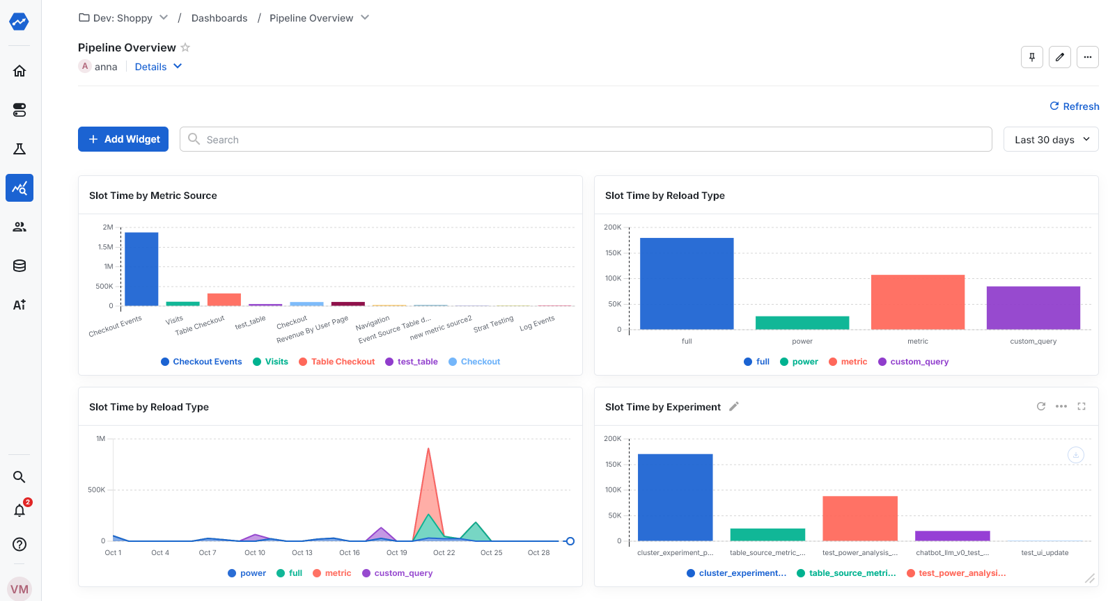
Statsig builds this dashboard with Statsig Product Analytics. You can customize any of these charts or build new ones. A useful addition is to include your average compute cost, so you can convert slot time per experiment into dollar cost per experiment.
At the end of every Pulse load / DAG, Statsig uploads a single row to the pipeline_overview table for each job executed as part of that run. This table has the following schema:
| Column | Type | Description |
|---|---|---|
| ts | timestamp | Timestamp at which the DAG was created. |
| job_type | string | Job type (see Pipeline Overview) |
| metric_source_id | string | Only applicable for 'Unit-Day Calculations' jobs - the ID of the metric source |
| assignment_source_id | string | The Assignment Source ID of the experiment for which Pulse was loaded. |
| job_status | string | The final state of the job (fail or success) |
| metrics | string | Metrics processed by the job |
| dag_state | string | Final state of the DAG (success, partial_failure, or failure) |
| dag_type | string | Type of DAG (full, incremental, metric, power, custom_query, autotune, assignment_source, stratified_sampling) |
| experiment_id | string | ID of the experiment for which Pulse was loaded, if applicable |
| dag_start_ds | string | Start of the date range being loaded |
| dag_end_ds | string | End of the date range being loaded |
| wall_time | number | Total time elapsed between DAG start and finish, in milliseconds |
| turbo_mode | boolean | Whether the DAG was run in Turbo Mode |
| dag_id | string | Internal identifier for the DAG |
| dag_duration | number | Number of days in the date range being loaded |
| is_scheduled | boolean | Whether the DAG was triggered by a scheduled run |
Was this helpful?