Cohort Metrics
Cohort metrics are a way to analyze the impact of an experiment in a certain time frame per experimental unit
Cohort metrics are useful for many reasons. Common use cases are:
- By ensuring all users have equal periods for data collection, there is an "apples to apples" comparison across user enrolled early/late in the experiment (which often corresponds to power/occasional users), and across different "time periods" that may have extrinsic factors like holidays
- If analyzing an unbounded period, experimental units' variance in the population can increase over time - leading to scenario where error bars don't actually converge towards 0 as the experiment is run for longer!
- This allows one to skip noisy early metrics, or focus on outcomes after users might churn - e.g. capturing "week-2 engagement" if a product has a 1-week trial period
- This can also be used to capture "one-shot retention". Retention metrics are used to capture rolling, ongoing retention. A user metric with a window from day X to day Y is a good way to check if an experiment is causing more users to retain at least X days
The downsides of cohort metrics are that:
- They don't capture any sort of long-term impact, or how that evolves over time. This is purely a point in time analysis and may not be appropriate for measuring complex, evolving behaviors
- They make topline impact estimates lossier and harder to trust
Some practitioners have made compelling arguments that cohort metrics are a better "standard" metric for organizations to use in analysis. Statsig tends to believe that the use of cohorts is dependent on business context, but consider whether they should be at least a part of an experiment's measurement (for example, measuring topline revenue as an overall evaluation criteria, but also measuring 7d revenue alongside it for additional context).
This page explains the available settings, what they do, and how they interact so you know what Statsig measures.
Basic cohort windows
Basic cohort windows are a filter on metric data with a time range relative to the unit's time of exposure. For example, a cohort window from day 1 to day 6 filters to events from 24 hours until 168 hours after exposure.
This is calculated as a timestamp comparison; a unit enrolled at 12pm will have exactly 24 hours until they hit the end of a 0-1 day cohort.
For metrics from data sources that are marked as daily data, the cohort comparison is truncated to a date so that day-0 data behaves as expected (e.g. a user exposed on 2025-01-05T09:00 will include the date-based data from 2025-01-05 instead of truncating to times "after 9:00am").
Waiting for maturation
By default, cohort metrics can have a mix of maturation levels in the experimental population. For a 1-week cohort, users enrolled in the final week have a mix of maturities during analysis. This yields the maximum sample but can dilute the analysis with partial cohort windows. To prevent this, mark the metric as "Wait for cohort window to complete". This drops units' metric data from analysis and removes them from the experiment analysis population.
In the examples below, one metric forces cohorts to complete. It has less units in the analysis, since many units don't have a complete window, a lower total because of the small unit count, but a higher mean since the units it does have have completed their window and have a longer data collection period on average.
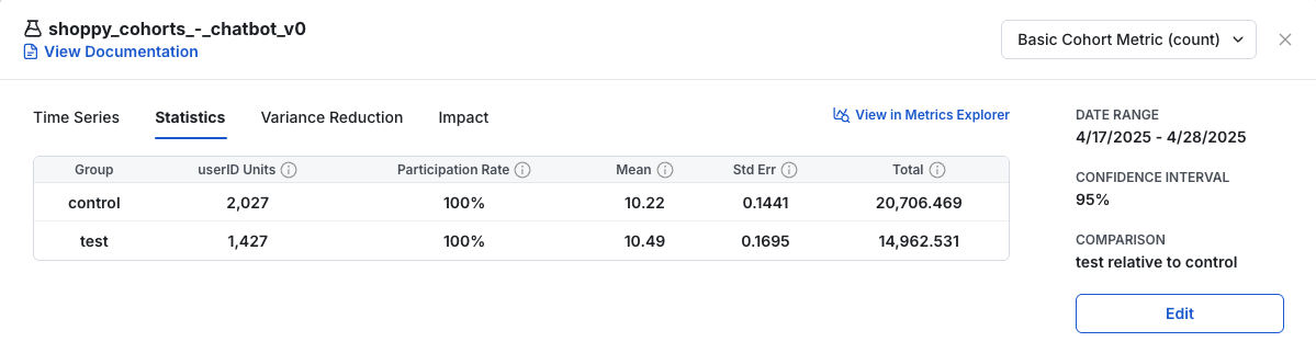
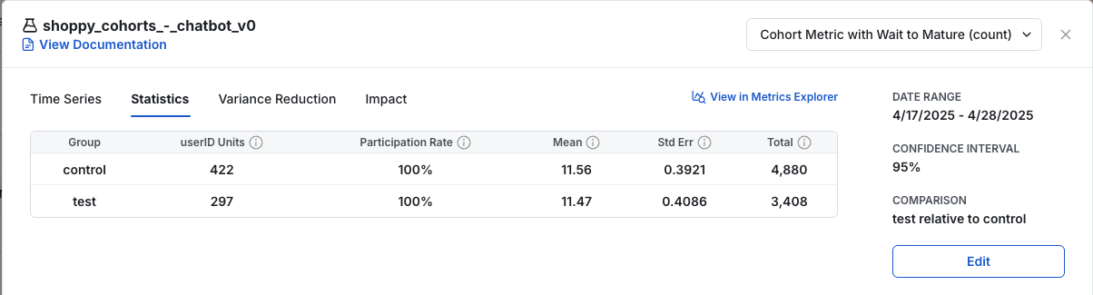
This setting can lead to different populations between metrics and filters out the last few days of an experiment's data in the daily time series, because new cohorts' data is not yet complete. View a metric's cohort settings by hovering over the metric name in the experiment scorecard.
Visual examples
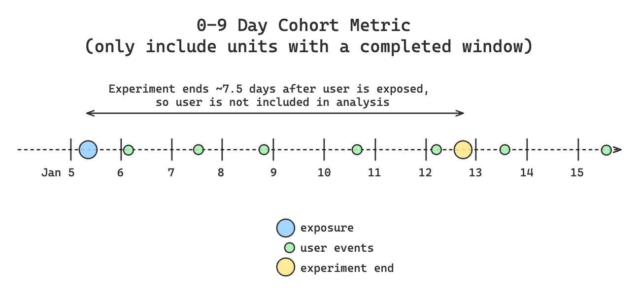
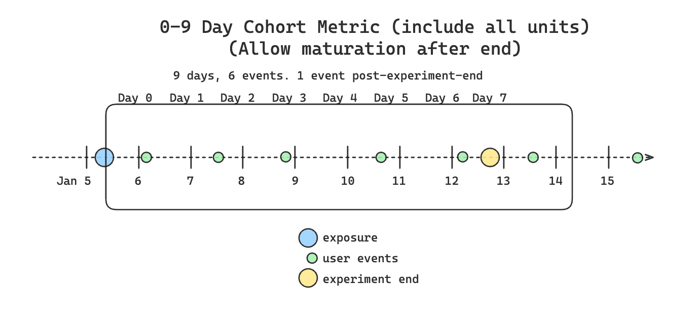
This is what data collection looks like for a standard cohort metric with a 0-6 day window. This collects data for 7 days because it is 0-indexed.
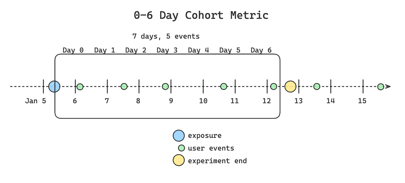
If the cohort period extends past the end of the experiment, data collection is truncated to the end of the experiment by default.
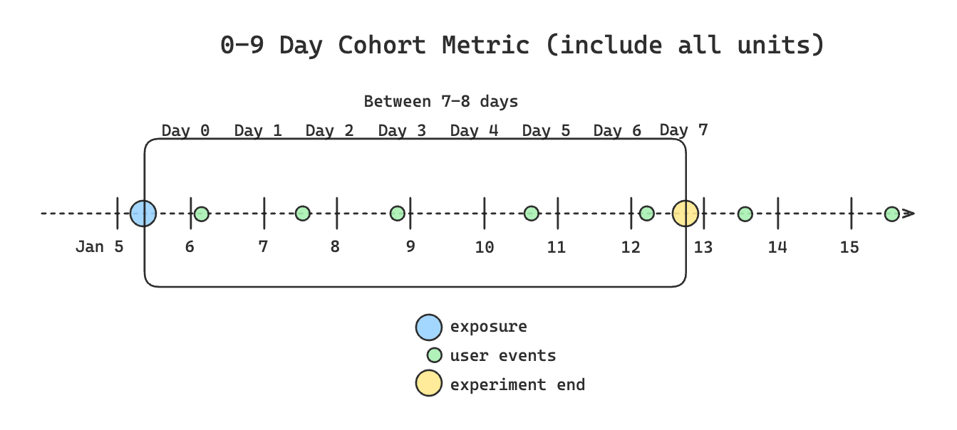
If the metric is configured to allow only completed cohort windows, Statsig excludes the unit from the analysis. Statsig doesn't include excluded units in the denominator for the average value of a sum or count metric, and filters their metric data from the analysis.
If mature after end is configured in the experiment, data collection continues after the experiment ends, regardless of whether "wait for mature" is enabled.
Experiment-based cohort settings
Cohort controls are also available at the experiment level. The relevance of these settings depends on the kind of experiment being run, as described below.
Allow post-experiment cohort data
Checking Allow Cohort Metrics to Mature After Experiment End allows metrics to be collected after the experiment ends. This is recommended for one-time interventions, such as a new signup page, because post-experiment signal from units that received the intervention provides additional statistical power.

This is not recommended for continuous interventions, such as a ranking change, because post-experiment data can be diluted. For example, test users may receive the control experience during their post-experiment period, which dilutes results.
The analysis is extended past the experiment end by the length of the longest cohort window across all metrics. Non-cohorted metrics are constrained to the analysis period; cohort metrics are filtered to the experiment end plus their cohort window.
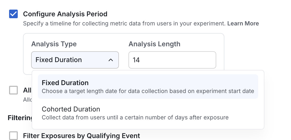
Fixed duration
On the Experiment Population section of the experiment setup page, Configure Analysis Period with Analysis Type Fixed Duration counts metrics only for a specified period after experiment start. This is useful for experiments with a fixed enrollment point, such as email campaigns.
This setting is only available for assign and analyze experiments.
Cohorted duration
On the Experiment Population section of the experiment setup page, Configure Analysis Period with Analysis Type Cohorted Duration applies allocation-based cohorting globally to all metrics in the experiment analysis. This is the same as the metric-based cohort but applied experiment-wide. This is useful for new user experiments.
When this is used in conjunction with metric cohorts, Statsig uses the minimal end of the cohort window. For example, if a metric cohort is set to end at 7 days and the experiment at 10 days, Statsig uses 7. If the metric cohort is set to end at 7 days and the experiment at 5 days, Statsig uses 5.
The only include units with a completed cohort window setting can also be specified at the experiment level and applies to all metrics in the experiment when set. If not checked, the setting is applied on a metric-by-metric basis.
Metric bake windows
In some cases, a metric in your warehouse may not be mature until a certain time has passed, after which you care about the daily value. Statsig provides the option to specify a bake window for your metrics. Statsig excludes metrics that haven't reached the end of their bake window from the numerator and denominator of the metric in the analysis.
Daily revenue is an example of a metric that may not be immediately mature. If a user makes a purchase and refunds it a few days later, their daily revenue retroactively changes to reflect the refund. A 28-day refund period would align naturally with a 28-day bake window for revenue metrics.
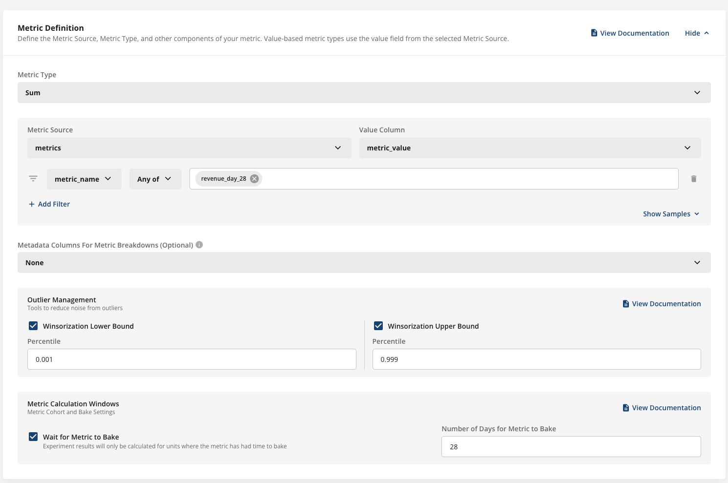
In the example above, the revenue metric covers the last 28 days. Rather than calculating a partial result, users are excluded from the analysis until their data has had 28 days to mature.
Partial results can occur because, when a metric bakes over a long period, part of the metric values come from before the experimental intervention and dilute the results. For a user exposed 1 day ago, 27 of 28 days of their revenue metric would be from the pre-intervention period, diluting the experiment results.
Was this helpful?