Metric drill-down

Drill down into Statsig experiment results by user segment, dimension, or time period to understand which sub-populations drive aggregate metric changes.

Metric drill-down shows the statistics behind a single Scorecard result: group sizes, means, totals, the p-value, the time series of the lift, and the projected topline impact. Use it when a metric moved and you need to see whether the effect is stable over time or driven by a small number of units. To break a metric down by a dimension, use a custom Explore query instead.

When you hover over a metric on the Results tab, Statsig shows a tooltip with key statistics.

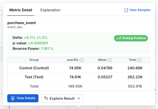
Group: The name of the group of users. For feature gates, Statsig treats the Pass group as the test group and the Fail group as the control. For experiments, these are the variant names.
Units: The number of distinct units included in the metric, for example distinct users for user_id experiments or devices for stable_id experiments.
Mean: The average per-unit value of the metric for each group.
Total: The total metric value across all units in the group, over the time period of the analysis.

Calculation details

Metric type	Total calculation	Mean	Units
`event_count`	Sum of events (99.9% winsorization)	Average events per user (99.9% winsorization)	All users
`event_user`	Sum of event DAU (distinct user-day pairs)	Average `event_dau` value per user per day. Statsig calls this "Event Participation Rate" because it represents the probability that a user is DAU for that event.	All users
`ratio`	Overall ratio: sum(numerator values)/sum(denominator values)	Overall ratio	Participating users
`sum`	Total sum of values (99.9% winsorization)	Average value per user (99.9% winsorization)	All users
`mean`	Overall mean value	Overall mean value	Participating users
user: `dau`	Sum of daily active users	Average metric value per user per day. The probability that a user is DAU.	All users
user: `wau`, `mau_28day`	Not shown	Average metric value per user per day. The probability that a user is xAU.	All users
user: `new_dau`, `new_wau`, `new_mau_28day`	Count of distinct users that are new xAU at some point in the experiment	Fraction of users that are new xAU	All users
user: retention metrics	Overall average retention rate	Overall average retention rate	Participating users
user: L7, L14, L28	Not shown	Average L-ness value per user per day	All users

p-value

In null hypothesis significance tests, the p-value is the probability that a difference as extreme as the observed one arises by random chance when the experiment has no actual effect. A p-value threshold determines which results count as a real effect and which are plausibly due to random chance. For the formula, refer to p-value calculation.

Reverse power

Reverse power is the smallest effect size that an experiment can reliably detect in its current state (some studies call this value ex-post MDE). Statsig calculates it from the sample size and the standard error of the control group. Reverse power doesn't depend on the observed effect size. In practice, it answers the question: given how the test turned out, what's the smallest effect you have sufficient power (typically 80%) to detect?

For a two-sided test, Statsig computes the reverse power for a metric X as:

Reverse Power = \frac{(Z_{1-\beta} + Z_{1-\alpha/2})}{\overline{X}_{\text{control}}}\times \sqrt{\frac{\mathrm{var}(\Delta \overline{X})}{N_{\text{control}}}} \times 100\%

For a one-sided test, Statsig computes the reverse power for a metric X as:

Reverse Power = \frac{(Z_{1-\beta} + Z_{1-\alpha})}{\overline{X}_{\text{control}}}\times \sqrt{\frac{\mathrm{var}(\Delta \overline{X})}{N_{\text{control}}}} \times 100\%

$\overline{X}_{\text{control}}$ is the mean metric value across control users.
$var(Δ\overline{X})$ is the population variance of delta.
$N_{\text{control}}$ is the observed number of units in the control group.
$Z_{1-\beta}$ is the standard Z-score for the selected power. Typically ${1-\beta}$ = 0.8 and $Z_{1-\beta}$ = 0.84.
$Z_{1-\alpha/2}$ and $Z_{1-\alpha}$ are the standard Z-scores for the selected significance level in a two-sided test and in a one-sided test.

Reverse power is an optional feature. To turn it on or off, go to Settings > Product Configuration > Experimentation > Organization.

Detailed view

Select View Details to open the detailed view for a metric. It contains three sections:

Time Series: How the metric evolves over time.
Raw Data: Group-level statistics.
Impact: How the experiment affects the metric.

Time series

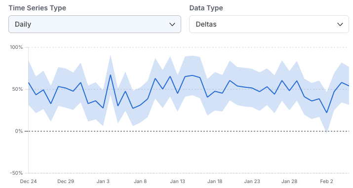
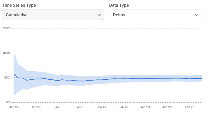
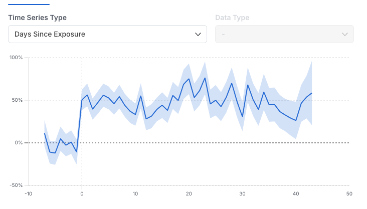
In the time series view, select and drag to zoom in on a time range. The drop-down offers three types of time series.

Daily

The metric impact on each calendar day, without aggregating days together. Use the daily view to assess day-over-day variability and the impact of specific events. It's the recommended view for holdouts because it highlights the impact over time as you launch new features.

Cumulative

The cumulative metric impact from the start of the experiment. Use the cumulative view to observe trends and to watch how the confidence interval changes over time.

Days since exposure

The metric impact based on how long a user has been in the experiment. Statsig aligns daily data for each user by the day the user entered the experiment (Day 0, Day 1, and so on), not by calendar date. This alignment lets you distinguish early (novelty) effects from long-term effects. This view also shows pre-experiment data, which reveals biases between groups before the experiment started. Such biases can arise from random chance or from an issue in the random assignment process.

Raw data

The raw data view shows the group-level statistics that Statsig uses to compute the metric deltas and confidence interval: Units, Mean, Total, and the standard error of the mean (Std Err). Refer to the statistical calculations reference for details.

Impact

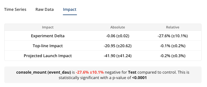
Experiment Delta (absolute): The absolute difference of the mean between groups, that is, Test Mean - Control Mean. Statsig shows the p-value to indicate whether the observed absolute difference is statistically significant.
Experiment Delta (relative): The relative difference of the mean, that is, 100% x (Test Mean - Control Mean) / Control Mean.
Topline Impact: The measured effect the experiment has on the overall topline metric each day, on average. Statsig computes it daily and averages it across the days in the analysis window. The absolute value is the net daily increase or decrease in the metric; the relative value is the daily percentage change.
Projected Launch Impact: An estimate of the daily topline impact Statsig expects if you launch the test group to all users. This estimate takes into account the layer allocation and the size of the test group, and assumes that the targeting gate (if there is one) stays the same after launch.

The projected launch impact is often smaller than the relative experiment delta because the experiment reaches only a subset of the users who contribute to the topline metric, and the topline impact can be higher or lower than the experiment delta because Statsig computes the two values differently (unit-level averages for deltas, daily pooled totals for topline). For the calculations, refer to topline and projected impact calculations.

Was this helpful?