What is Switchback Testing?
Switchback tests are an alternative experiment form, whereby an entire population is “switched” back and forth between test and control treatments on a set cadence vs. being split and evenly divided between test and control for the duration of the experiment. Switchback tests are particularly common in marketplaces, whereby running a traditional A/B on one side- or a small %- of the marketplace would have an unintended consequence on the rest of the marketplace due to network effects, ultimately impacting experiment results. Another common use case for switchbacks occurs when applying different variants to different users is infeasible for fairness, legal, or logistical reasons. Switchback tests are often carried out across multiple “buckets”, typically regions or other defined groups that are flipped between test and control treatments over the course of the experiment.Example
Let’s say you are a rideshare platform and want to test pricing. You initially consider splitting your riders into two groups, one with the higher price and one with a lower price. However, you quickly notice that the riders with the lower price are requesting rides at a significantly higher rate, and sucking up all the available driver supply in a given area. This leaves the riders with higher prices with not only a higher ride estimate, but longer ETAs when they open up their app, making them even less likely to request. When you look at your experiment results you’re not sure if the decreased ride request rate in the higher price group was due to the higher prices they saw or the fact that their ETAs went up- your experiment results are polluted! You’ve inadvertently introduced bias to your results via your experimental design. In this scenario, you could consider running a Switchback test on your marketplace. To do this, you might switch 100% of your riders and drivers in a given metro in and out of the new pricing plan hourly and understand the impact on overall ride request rates during hours at which rider prices were higher vs. lower.Switchback Testing on Statsig
Methodology
Our Switchback Testing methodology for computing results consists of 3 steps:- Attribute events to the corresponding switchback bucket, where each bucket is defined by the time window and grouping attribute.
- Calculate the variant-level and bucket-level metrics based on the attributed events.
- Calculate the difference in means between test and control. Use bootstrapping to obtain the confidence intervals.
Event Attribution
Attribution of events to a particular bucket is based on the timestamp and unit_id of the exposure, the length of the attribution window, and the timestamp of subsequent events for that unit_id. For example: User 123 is exposed to bucket A at 9:15 am. The test has an attribution window of 90 minutes. This means all events triggered by user 123 between 9:15 am and 10:45 am will be included in the metric calculations for bucket A.Bucket-level Metrics
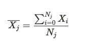
Once we have all the events corresponding to a bucket, we calculate the scorecard metrics derived from these events.
Variant-level Metrics
Similarly, we calculate the overall metric means for test and control by aggregating the values across all the buckets in that variant. So if there are M buckets in the test group, the mean value of a ratio metric is given by:

Deltas and Confidence Intervals
The treatment effect is calculated as: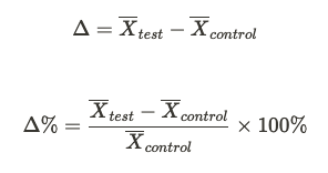
- Collect a bootstrap sample with replacement from the set of test buckets and separately from the set of control buckets.
- Calculate the difference in means between test and control samples.
- Repeat steps one and two 10 thousand times. This gives us a distribution of the metric deltas
- The 95% confidence interval is the range from the 2.5% quantile to the 97.5% quantile from the distribution of deltas in step three. In general, the confidence interval with significance level is given by

Setup
To set up a Switchback test on Statsig, when you create an experiment tap Advanced Settings → Experiment Type and select “Switchback Test”.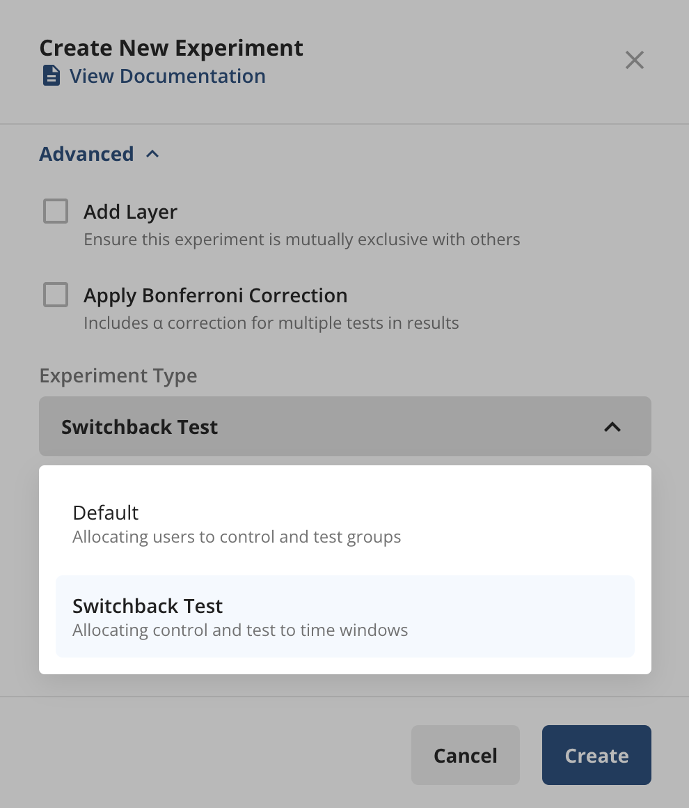
- Targeting- The defined population(s) you will be running your experiment on.
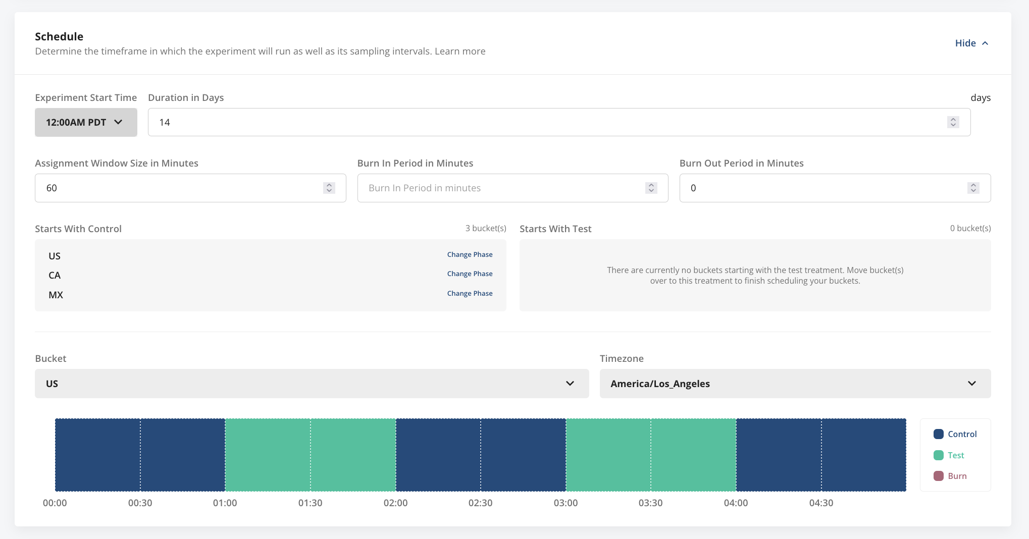
- Schedule- The switching frequency and starting treatments for different pre-defined populations.
- Targeting Gate- Specify a targeting gate to define your target experiment population, similar to any other experiment on Statsig.
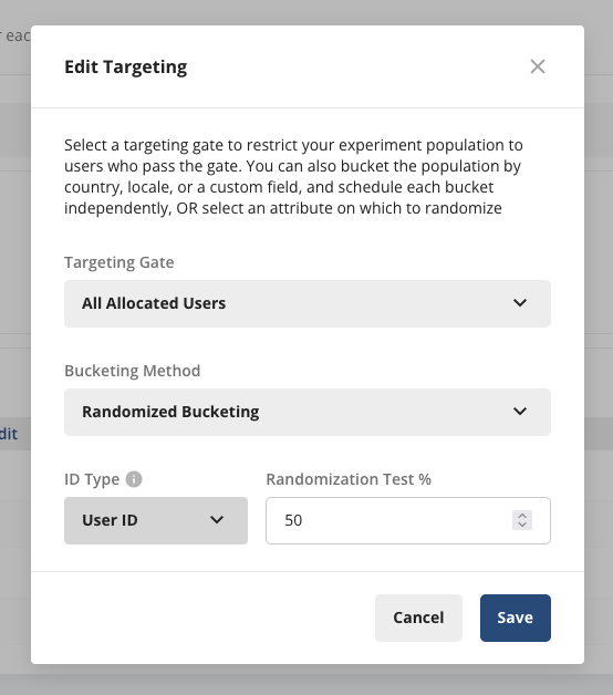
- Bucketing Method- Bucket users based on either pre-defined buckets or randomized across an ID type.
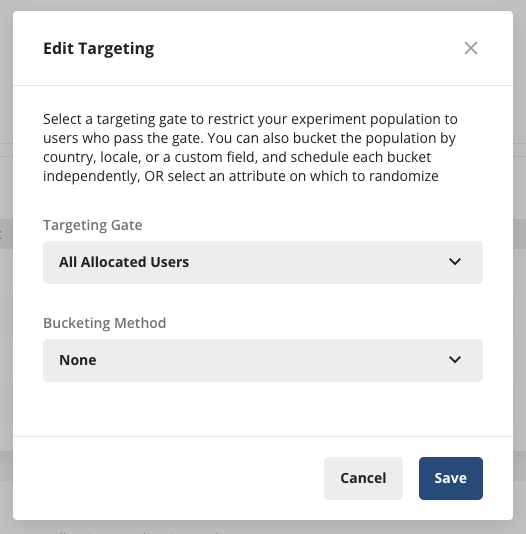
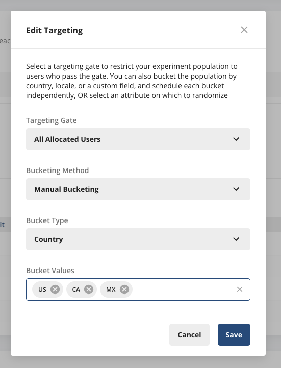
Randomized bucketing is an advanced feature, please reach out to our support team, your sales contact, or via our Slack community if you want this enabled.
- Start time
- Duration (in days)
- Assignment window size (in minutes)
- Burn-in/ burn-out periods (in minutes)
- (Pre-defined bucketing only) Starting phase (treatment group) for each bucket
Reading Results
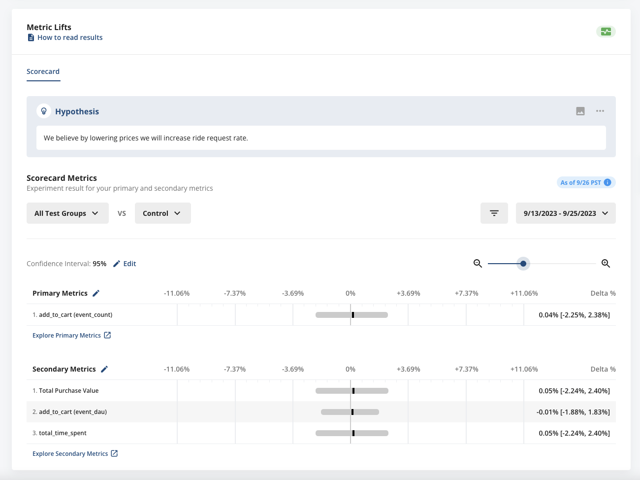
Both Diagnostics and Pulse metric lifts results for Switchback tests will look and feel like Statsig’s traditional A/B tests, with a few modifications-- No hourly Pulse- At the beginning of a traditional A/B/n experiment on Statsig, you can start to see hourly Pulse results flow through within ~10-15 minutes of experiment start. Given in a Switchback you will only see either all Test or all Control exposures right at experiment start, we have disabled Hourly Pulse until you have a meaningful amount of data. However, in lieu of Hourly Pulse you can still leverage the more real-time Diagnostics tab to verify checks are coming in and bucketing as expected.
- No time-series- The Daily and Days Since First Exposure time-series are not available for Switchback tests. This is due to the bootstrapping methodology used to obtain the statistics, which relies on pooling all the available days together in order to have enough statistical power.
- No dimension breakdown- Breaking down a metric by user property or event property is not available for Switchback tests.
- Advanced statistical techniques- CUPED and Sequential Testing are not yet available on Switchback tests.
