Frequentist Sequential Testing

What's the problem with looking early in a "standard" A/B test?

Traditional A/B testing best practices (t-tests, z-tests, etc.) dictate that the readout of experiment metrics should occur only once, when the target sample size of the experiment has been reached (i.e. your design duration has been reached and you reach the desired sample size). We call this a "Fixed Horizon Test", because when designing an experiment you set the amount of desired units you wish to observe and (ideally) commit to analyzing the results only once this dataset is complete.

Continuous experiment monitoring (i.e. "peeking") for the purpose of decision making, however, results in inflated false positive rates (a.k.a. the peeking problem) which can be much higher than that expected from your desired significance level.

How does peeking increase decision error rates?

Continuous monitoring leads to inflated false positives because any time you consider ending an experiment early you are at risk of making a conclusion that is incorrect. Remember, at the core of a standard hypothesis test, you are deciding if you should "accept the null" hypothesis or "reject the null" hypothesis and accept the alternative. As an A/B practitioner, you must decide between rejecting or not rejecting the null. Any time you look early and allow the possibility of making a decision early, you are potentially rejecting the null hypothesis even when the null hypothesis is actually correct.

Why would early results be "wrong"?

Metric values and p-values always fluctuate to some extent due to noise during any experiment, and results can transition into and out of statistical significance due to this noise, even when there is no real underlying effect. These noisy fluctuations can be caused by random unit assignment and random human behavior we can't predict, and the effects can't be entirely removed from an experiment. Not every test is subject to the same amount of experimental noise, however, and like so many things it's dependent on what you're testing and who your users are. Tests also vary over time in the amount of noise they see, especially as adding more users and observing them for longer tends to help the random fluctuations even out.

Peeking, however well-intentioned, will always introduce some amount of selection bias if we adjust the date of a readout. When an experimenter makes any early decision about results (e.g. "is the result stat-sig, can we ship a variant early?") they've increased the chances that their decision is based on a temporary snapshot of always fluctuating results. They are potentially cherry-picking a stat-sig result that might never be seen if the data were analyzed only once at the full, pre-determined completion of the experiment. Unfortunately, when running frequentist A/B test procedures this early decision can only increase the false positive rate (declaring an experimental effect when there really is none), even when the intention is to make a less-biased decision based on the statistics.

What is Sequential Testing for an A/B test?

In the variety of Sequential Testing on Statsig, the experimental results for each preliminary analysis window are adjusted to compensate for the increased false positive rate associated with peeking. Statsig adjusts your p-values and confidence intervals automatically, and you can see this in the Results tab:

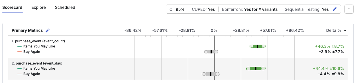
In this example, the confidence intervals for each metric are expanded using the "wings" or "tabs". This serves as a quick visual indicator that sequential testing is enabled and shows you how much the intervals have been expanded.

In this real-world example, you can see for the indicated result that the sequential testing adjust makes the difference between declaring the result stat-sig or not.

The goal of Sequential Testing is to enable early decision making when there's sufficiently strong observations that outweigh the random fluctuations while limiting the risk of false positives. While peeking is typically discouraged, regular monitoring of experiments with sequential testing is particularly valuable in some cases. For example:

• Unexpected regressions: Sometimes experiments have bugs or unintended consequences that severely impact key metrics. Sequential testing helps identify these regressions early and distinguishes significant effects from random fluctuations.
• Opportunity cost: This arises when a significant loss may be incurred by delaying the experiment decision, such as launching a new feature ahead of a major event or fixing a bug. If sequential testing shows an improvement in the key metrics, an early decision could be made. But use caution: An early stat-sig result for certain metrics doesn't guarantee sufficient power to detect regressions in other metrics. Limit this approach to cases where only a small number of metrics are relevant to the decision.

tip

Sequential testing can be used anywhere you do an experimental analysis. This includes your main experimental Results page as well as any custom queries.

Quick Guides

Enabling Sequential Testing Results

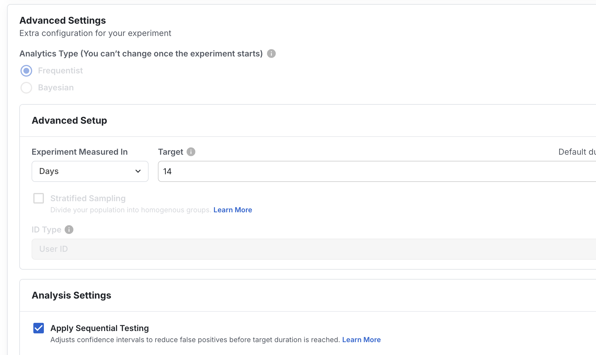
In the Setup tab of your experiment, with Frequentist selected as your Analytics Type, you can enable Sequential Testing under the Analysis Settings section. This setting can be toggled at any time during the life of the experiment, and it does not need to be enabled prior to the start of the experiment.

Interpreting Sequential Testing Results

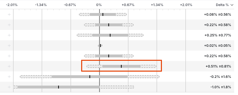
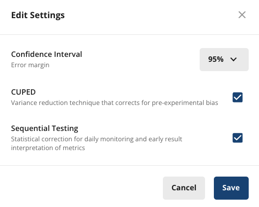
Click on Edit at the top of the metrics section in Pulse to toggle Sequential Testing on/off.

When enabled, an adjustment is automatically applied to results calculated before the target completion date of the experiment.

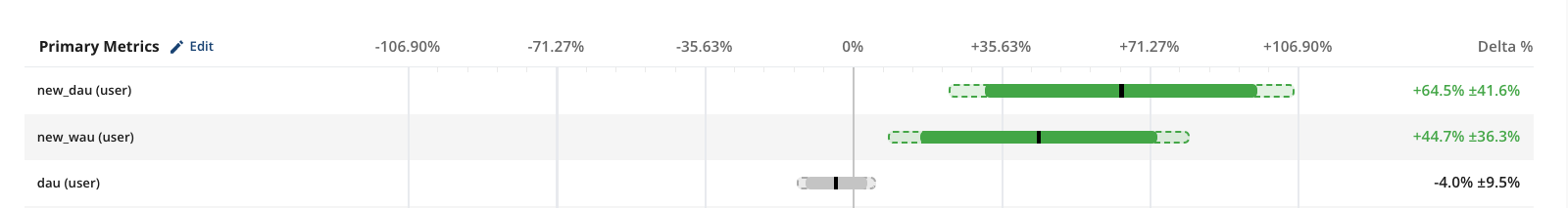
The dashed line represents the expanded confidence interval resulting from the adjustment. The solid bar is the standard confidence interval computed without any adjustments. If the adjusted confidence interval overlaps with zero, this means the metric delta is not stat-sig at the moment, and the experiment should continue its course as planned.

Sequential testing is a reliable way to make an early decision, particularly for early detection of regressions. One should be mindful that early decision-making will often result in underpowered lift estimates with a high degree of uncertainty. If making the right decision is important, you can use statistically-significant sequential testing results. If an accurate measurement is important, you should wait for full power as estimated by your pre-experimental power calculation. We do not calculate statistical power on post-hoc experimental results (See section "Post-hoc Power Calculations are Noisy and Misleading" in Kohavi, Deng, and Vermeer, A/B Testing Intuition Busters.

Statsig's Implementation of Sequential Testing

Two-Sided Tests

Confidence Intervals

Statsig uses mSPRT based on the the approach proposed by Zhao et al. in this paper. The two-sided Sequential Testing confidence interval with significance level $\alpha$ is given by:

$$CI^*(\Delta \overline{X}) = \Delta \overline{X} \pm Z^*_{\alpha/2} \cdot \sqrt{V}$$

where

• $Z^*_{\alpha/2}$ is the z-critical value, modified for sequential testing:

$$Z^*_{\alpha/2} = \sqrt{\frac{(V+\tau)}{\tau}\left(-2\ln(\alpha/2)-\ln(\frac{V}{V+\tau})\right)}$$

• $V$ is the standard variance of the delta of means when computing variance. It can be obtained from the sample variance of the test and control group means:

$$V = var(\Delta \overline X) = var(\overline X_t) + var(\overline X_c) = \frac{var(X_t)}{N_t} + \frac{var(X_c)}{N_c}$$

• $\tau$ is the mixing parameter given by:

$$\tau =(Z_{\alpha/2})^2\cdot\frac{var(X_t)+var(X_c)}{N_t+N_c}$$

• $Z_{\alpha/2}$ is the z-critical value used in the non-sequential test, for the desired significance level (1.96 for the standard $\alpha = 0.05$)

We have validated that this parameter satisfies the expected False Positive Rate and provides enough power to detect large effects early. More details on this analysis are available here.

p-Values

It's possible to produce p-values for sequential testing that are consistent with the expanded confidence intervals above by modifying our p-value methods.

We want to evaluate the mSPRT test so that our Type I error remains approximately equal to $\alpha$, and so that the sequential testing p-value is consistent with the expanded confidence interval. (I.e. A CI that includes 0.0% should have p-value ≥ $\alpha$, and one that excludes 0.0% should have p-value < $\alpha$.)

Our observed z-statistic (i.e. z-score) remains unchanged. Instead of evaluating $Z$ on a standard-normal distribution $N(0, 1)$ as we usually do, we evaluate against some other normal distribution $N(0, \sigma^2)$ with mean of zero and standard deviation $\sigma$. For a two-sided test, since we want the probability of an observed $Z$ exceeding $Z^*_{\alpha/2}$ (assuming the null hypothesis to be true) to be limited to $\alpha$, we can find the unknown parameter by solving for $\sigma$:

$$\sigma=\frac{Z_{\alpha/2}^*}{\sqrt{2} \cdot erf^{-1}(1-\alpha)}$$

where $erf^{-1}$ is the inverse error function.

From here we can compute the two-sided sequential testing p-value as:

$$\text{p-value}^* = 2 \cdot \frac{1}{\sqrt{2\pi}} \int \limits _{-\infty}^{-|Z|} \frac{e^{- \frac{t^2}{{2\sigma^2}}}}{\sigma}dt$$

where $Z$ is the observed z-statistic (i.e. z-score) as usual.

One-Sided Tests

We can modify each step for one-sided sequential testing.

$$CI^*(\Delta \overline{X}) = \begin{cases} \left[\Delta \overline{X} - Z^*_{\alpha} \cdot \sqrt{V}, \quad +\infty \right) & \text{if right-sided test} \\ \\ \left(- \infty, \quad \Delta \overline{X} + Z^*_{\alpha} \cdot \sqrt{V} \:\right] & \text{if left-sided test} \\ \end{cases}$$ $$\text{p-value}^* = \begin{cases} 1 - \frac{1}{\sqrt{2\pi}} \int \limits _{-\infty}^{Z} \frac{e^{- \frac{t^2}{{2\sigma^2}}}}{\sigma}dt \quad \text{if right-sided test} \\ \\ \frac{1}{\sqrt{2\pi}} \int \limits _{-\infty}^{Z} \frac{e^{- \frac{t^2}{{2\sigma^2}}}}{\sigma}dt \quad \text{if left-sided test} \\ \end{cases}$$

where

• $Z^*_{\alpha}$ is the one-sided test z-critical value, modified for sequential testing:

$$Z^*_{\alpha} = \sqrt{\frac{(V+\tau)}{\tau}\left(-2\ln(\alpha)-\ln(\frac{V}{V+\tau})\right)}$$

• $V$ is the the same as for two-sided tests.

• $\tau$ is the mixing parameter given by:

$$\tau =(Z_{\alpha})^2\cdot\frac{var(X_t)+var(X_c)}{N_t+N_c}$$

• $Z_{\alpha}$ is the one-sided z-critical value used in the non-sequential test, for the desired significance level (1.645 for the standard $\alpha = 0.05$)

• $\sigma$ is solved via:

$$\sigma = \begin{cases} \frac{Z_{\alpha}^*}{\sqrt{2} \cdot erf^{-1}(1 - 2 \alpha)} & \text{if right-sided test} \\ \\ \frac{- Z_{\alpha}^*}{\sqrt{2} \cdot erf^{-1}(2 \alpha - 1)} & \text{if left-sided test} \end{cases}$$

• $Z$ is the (signed) observed z-statistic as usual (i.e. z-score)