Contextual Bandit Methodology
Methodology behind Statsig Contextual Bandits, including the contextual algorithm, exploration strategy, model retraining, and reward attribution.
How contextual bandits work
Statsig runs contextual bandits with the same high-level approach across cloud and Warehouse Native deployments. Implementation details change frequently as Statsig experiments and optimizes its approaches, so this documentation stays intentionally high-level.
Core approach
The implementation follows the disjoint model methodology from Li, Chu, Langford, Schapire. Statsig trains one model per variant and computes estimated confidence intervals (CIs) for each. When you trigger contextual autotune, the latest model version estimates the user's outcome and adds the upper end of the 95% CI to that estimate.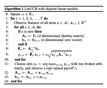
Statsig models categorical outcomes as logistic regression with L2 penalty. Statsig models continuous outcomes as multivariate ridge regression.
Training data and sampling
To keep data relevant, Statsig upsamples contextual autotune data to prefer recent dates. Sampling uses these mechanisms:
- Statsig selects a flat number of samples, preferring the most recent records.
- Per day, over the last two weeks, Statsig chooses samples to prefer more recent records.
- Statsig strictly prefers samples from the explore dataset, but may use non-explore data to satisfy sample requirements. Statsig then prioritizes records by a unit-ID hash to maintain stability in the training set between runs and avoid major jitter.
- Statsig chooses a sample set per variant to avoid bias from a dominant model being overrepresented in the training data.
If a model has very low volume, it has low representation in the training data. Lower representation causes higher CIs, which increases the upper bound and makes Statsig more likely to select that variant. This acts as a bounce-back mechanism for low-traffic variants.
Model and feature updates
Statsig updates models hourly. If a model definition changes (features or target outcome), Statsig resets all data, and the model retrains to match the new definition on the next hourly update.
The pre-training data pipeline appears in the history view on the results page, showing the SQL used and the caching tables where Statsig stores data. You can use this data to validate or explore modeling approaches.
Feature encoding
Statsig treats features with numerical-only values as continuous random variables. Statsig string-encodes and one-hot-encodes all others into binary variables for regression, using the top 25 levels available in the data with more than 1% coverage.
Statsig doesn't support arrays of categories or tags, or encodes only the most common tag sets. Provide tags as individual key-value pairs in the user custom object instead.
Model monitoring
Statsig doesn't offer diagnostics for model characteristics over time. Model coefficients are visible in the results tab. You can view a comparison of performance between naive random traffic and targeted traffic to determine whether model performance relative to blind allocation improves or degrades over time.
Was this helpful?