Switchback V2
Run switchback experiments in Statsig to alternate treatment exposure across time windows for marketplace, ranking, and other globally shared systems.
What is a switchback experiment?
A switchback experiment tests two versions of a system by alternating them over time. This methodology is useful when it isn't possible to isolate user experiences between treatment and control groups.
For example, on a rideshare platform, offering lower prices to a treatment group might increase demand for cars and indirectly affect control riders. A switchback experiment measures impact over time by alternating between experiences instead of splitting users.
How switchback experiments work
At a high level, switchback experiments work as follows:
Define clusters and their schedule: A cluster is a group of users that switch between experiences on the same cadence.
Example: All users in New York and Chicago follow this schedule:
- 9:00–10:00 AM: Control
- 10:00–11:00 AM: Treatment
- 11:00 AM–12:00 PM: Control
- 12:00–1:00 PM: Treatment
Aggregate data by time buckets: A bucket represents a single window of time during which the user experience remains constant. The analysis treats each bucket as one data point.
Example: In the schedule above, the experiment produces four buckets: two for control and two for treatment.
- Control
- Bucket 1: 9:00–10:00 AM
- Bucket 3: 11:00 AM–12:00 PM
- Treatment
- Bucket 2: 10:00–11:00 AM
- Bucket 4: 12:00–1:00 PM
- Control
Run regression analysis: Statistical models account for factors such as time of day, day of week, or cluster attributes when estimating the difference between treatment and control.
Compare results: The final output resembles a traditional A/B test, including metrics such as estimated lift and confidence intervals.
Setting up a switchback experiment
Defining the hypothesis, metrics, groups, targeting, and parameters follows the same general workflow as a traditional A/B test. Switchback experiments add three additional configurations: clusters, scheduling, and analysis configuration.
Defining cluster(s)
Clusters are groups of users who follow the same experience cadence. In traditional A/B tests, the selected ID Type acts as both the randomization unit and the unit at which Statsig calculates metrics. In a switchback experiment, however, the ID Type defines the unit for metric calculation. Clusters determine which experience a user receives over time.
Statsig provides three ways to define a cluster.
| Method | Description | Inputs |
|---|---|---|
| Single | Single Cluster where all users eligible for the experiment follows the same cadence | Start With: defines which experience (control or treatment) starts the switchback |
| Auto | Provides a two-cluster configuration where Statsig automatically assigns users to each cluster based on the specified inputs. | Cluster ID Type: Select a custom ID from the Exposure User Object that Statsig uses to split users into clusters. For example, if server_id is present on the user object, Statsig randomly assigns server_id values to each cluster, and groups users based on their server_id. |
| Manual | Two-cluster configuration where users are manually assigned to each cluster. | Cluster Field: Select a field from the Exposure User Object that Statsig uses to assign users to clusters. For example, if Country is selected as the Cluster Field, you can assign specific countries to either Cluster 1 or Cluster 2. Statsig then places users into clusters based on the value of that field (for example, their country). |
You can use the Cluster ID Type (Auto) and Cluster Field (Manual) fields as covariates in the regression analysis, and to break down metric data in the results section.
Defining scheduling
After you configure the clusters, you can define the schedule for experiences within each cluster.
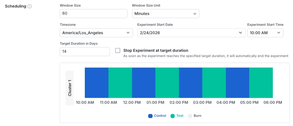
Inputs
Window Size / Unit: The length of each window during which a user’s experience remains constant.
Experiment Start Date / Time / Timezone: The date and time when the switchback experiment begins. All clusters start simultaneously. You can't start the experiment if the selected start date or time is in the past when the experiment starts.
Target Duration: The intended length of time the experiment should run. By default, the experiment doesn't automatically stop when it reaches this duration. Users continue to receive the switched experiences according to the configured schedule. If you enable ”Stop Experiment at target duration”, the experiment stops automatically at the end of the specified duration. After the experiment stops, Statsig serves users the default experiment value configured in code.
Define analysis configuration
You can configure how Statsig handles exposures and metrics during the transition periods between switchback windows. For example, a rideshare marketplace might switch from Control to Treatment at 9 AM. The system may still experience lingering effects from the Control period, such as drivers already on active trips or riders remaining in the queue from earlier periods. In these cases, you may want to exclude exposures and metric data recorded shortly after the switch.
Configure Burn-in and Burn-out periods in the Analysis Configuration section to exclude these transition exposures.
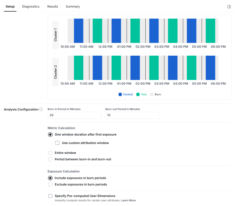
Inputs
Burn-in Period: The amount of time at the beginning of each window that Statsig excludes from analysis.
Burn-out Period: The amount of time at the end of each window that Statsig excludes from analysis.
Metric Calculation: Determines how Statsig attributes metric events to an exposure. The following options define how Statsig aggregates metrics within each switchback window.
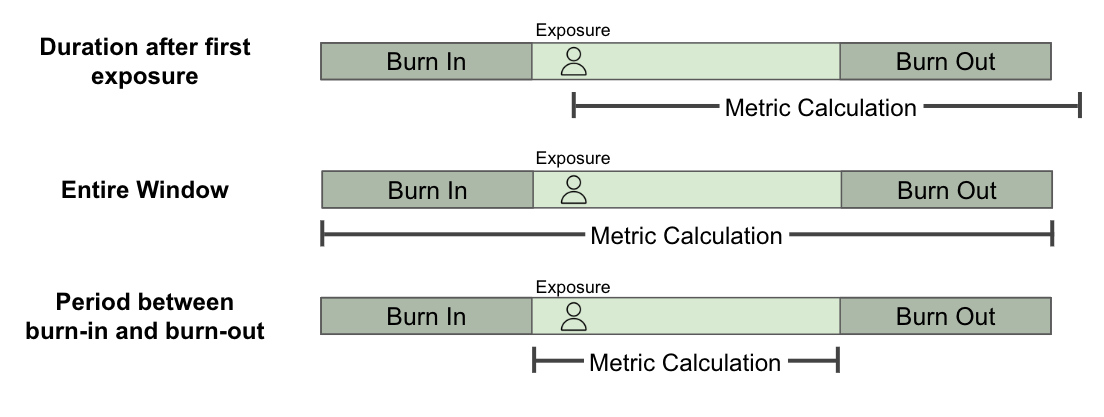
- Period from first exposure: Aggregates metric data for a specified period of time after the user’s first exposure.
- Entire window: Aggregates metric data across the full switchback window.
- Period between burn-in and burn-out: Aggregates metric data only within the portion of the window between the burn-in and burn-out periods.
Exposure Calculation: Defines how Statsig handles exposures logged during switchback windows in the analysis. Statsig offers the following options:
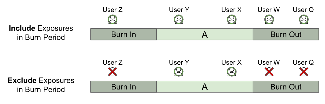
- Include exposures in burn periods: Considers all exposures recorded during the switchback window, including those that occur within the burn-in and burn-out periods.
- Exclude exposures in burn periods: Considers only exposures recorded between the burn-in and burn-out periods.
[Coming soon] Specify Pre-computed User Dimensions: Configure user dimensions to break down experiment results in the results section. You select these fields from the exposure user properties or entity properties.
Was this helpful?