For AI agents: a documentation index is available at /llms.txt. Append .md to any page URL for markdown, or send Accept: text/markdown.
Bonferroni Correction
How Statsig applies the Bonferroni correction to adjust p-values when testing multiple metrics or comparisons in an experiment to control false positives.
Bonferroni correction divides an experiment's significance level () by the number of comparisons, so the chance of any false positive across all metrics and variants stays at . That chance is the family-wise error rate. The Benjamini-Hochberg (BH) procedure instead controls the false discovery rate, the share of significant results that are false positives. BH therefore rejects more null hypotheses than Bonferroni for the same p-values. Use BH when a scorecard has many metrics and a small, controlled share of false positives is acceptable. Use Bonferroni when any single false positive is costly.
If you run a test with = 0.05, the probability of a false positive is 5%. Each additional comparison at the same significance level is another opportunity for a false positive, so the chance of at least one false positive grows with the number of comparisons.
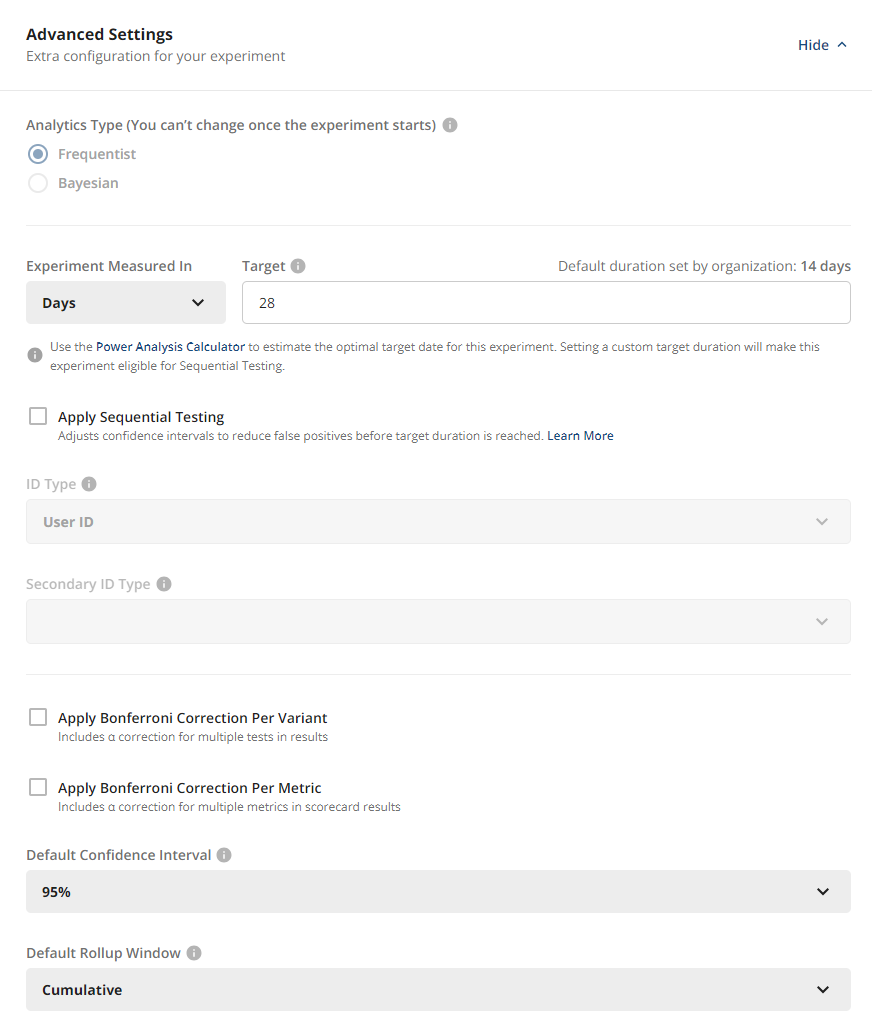
Bonferroni correction is an optional setting on Statsig experiments.
How Bonferroni divides the significance level
You can apply Bonferroni correction based on one or both of the following:
- Test groups (multiple treatment hypotheses): Statsig divides the significance level by the number of variants it compares against control.
- Metrics in the scorecard: You select what percentage of your total Statsig divides evenly among the primary metrics. Statsig splits the remaining equally among the secondary metrics.
If you select both corrections, Statsig applies them together: after dividing among the metrics, Statsig divides each metric's by the number of test groups.
The following example applies the metric correction with a significance level of 0.05 and 60% of assigned to primary metrics:
| Tier | Count | share | Per-metric |
|---|---|---|---|
| Primary metrics | 2 | 60% | 0.6 * 0.05 / 2 = 0.015 |
| Secondary metrics | 4 | 40% | 0.4 * 0.05 / 4 = 0.005 |
To also correct for 2 test groups in this example, Statsig divides each per-metric by 2.
When you analyze dimensions with the metric correction enabled, Statsig applies the correction separately for the dimensional breakdown. Statsig uses the number of dimensions as the total metric count for the dimensional analysis. This doesn't affect top-line metrics.
How the adjusted significance level appears in experiment results
In the experiment scorecard, Statsig derives confidence intervals for applicable metrics from (1 - adjusted ). Hovering over a confidence interval displays the adjusted alongside other metric details.
In the experiment explore section, Statsig calculates a new adjusted based on your selections, and the confidence intervals use (1 - adjusted ).
Was this helpful?