Frequentist Sequential Testing

Sequential testing adjusts p-values and confidence intervals so you can read experiment results before the target sample size without inflating the false positive rate. Statsig implements it as a mixture sequential probability ratio test (mSPRT): each metric's confidence interval widens by an amount that shrinks as data accumulates. Use it on frequentist experiments when you need to catch regressions early or ship early on a statistically significant result.

Statsig offers three analysis methods, which you choose with the Analytics Type setting under Advanced Settings on the experiment Setup tab. Use frequentist analysis with sequential testing for standard p-values and confidence intervals that stay valid when you read results early. Use SPRT when you want unlimited peeking and the option to accept the null hypothesis as well as reject it. Use Bayesian mode for chance-to-beat and expected-loss readouts, with optional priors from past experiments.

Why peeking inflates false positives

Traditional A/B tests (t-tests and z-tests) are fixed-horizon tests. When you design the experiment, you set the number of units to observe, and you read the metrics once, after you reach that target sample size. Sequential testing lets you read results and make valid decisions before that point.

Continuous monitoring of an experiment, or peeking, inflates the false positive rate above the significance level you chose. Every time you consider ending an experiment early, you decide whether to reject the null hypothesis, and that decision can be wrong. Metric values and p-values fluctuate because of noise from random unit assignment and unpredictable user behavior, so results can move into and out of statistical significance even when there is no real effect. Noise levels vary by test and decrease over time as more users join and you observe them longer.

When you decide based on an early snapshot, you're more likely to select a statistically significant result that wouldn't appear if you analyzed the data once at the planned end of the experiment. In frequentist procedures, early decisions can only increase the false positive rate, even when you intend to make a less biased decision.

How sequential testing works for an A/B test

Statsig automatically adjusts p-values and confidence intervals for each preliminary analysis window to compensate for the increased false positive rate that peeking introduces. The Results tab shows the adjustment:

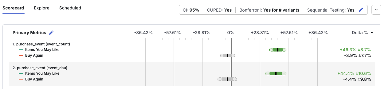
Statsig expands the confidence interval for each metric and marks the expansion with wings on the ends of the bar. The wings show that sequential testing is on and how much the interval expanded.

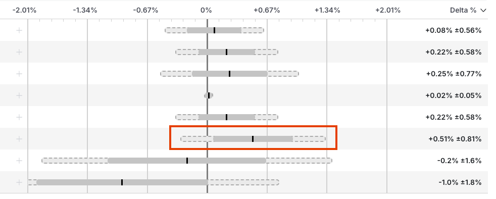
In this example, the sequential testing adjustment determines whether Statsig declares the result significant.

Sequential testing supports early decisions when observations are strong enough to outweigh random fluctuations, while limiting the risk of false positives. Statsig discourages peeking in general, but regular monitoring with sequential testing is valuable in two cases:

• Unexpected regressions: When an experiment has a bug or an unintended consequence that severely affects key metrics, sequential testing identifies the regression early and distinguishes significant effects from random fluctuations.
• Opportunity cost: Delaying a decision can be costly, for example when you need to launch a feature ahead of a major event or fix a bug. Sequential testing can support an early decision if key metrics show improvement. Use caution: an early significant result on some metrics doesn't guarantee enough power to detect regressions in other metrics. Limit this approach to cases where only a small number of metrics matter to the decision.

Enable sequential testing

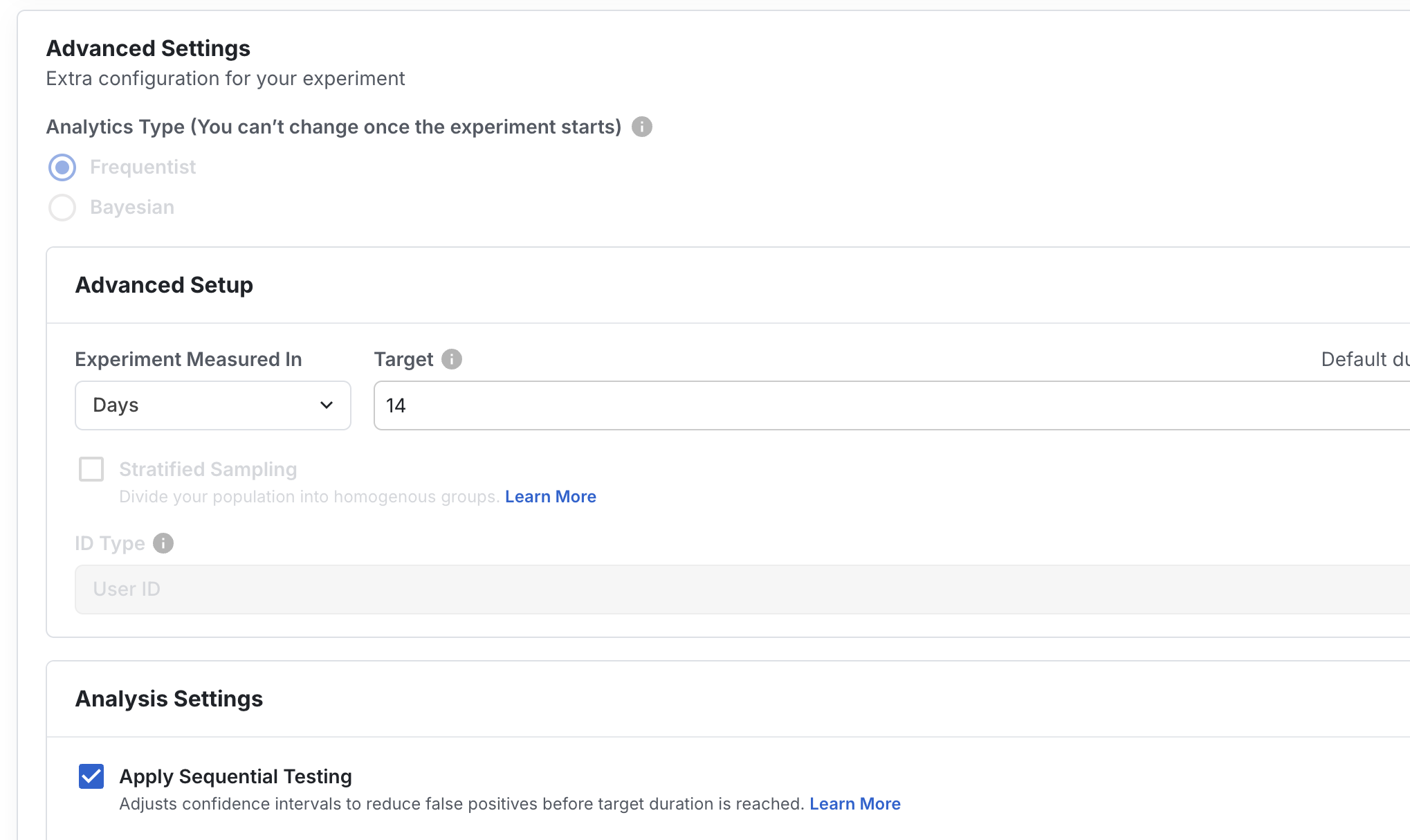
On the Setup tab of your experiment, set Analytics Type to Frequentist, then select Apply Sequential Testing under Analysis Settings. You can toggle this setting at any time during the experiment; you don't need to turn it on before the experiment starts.

Interpret sequential testing results

Click Edit at the top of the metrics section in Pulse to toggle sequential testing on or off.

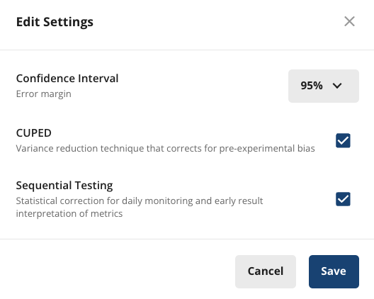
When you turn on sequential testing, Statsig adjusts the results it calculates before the target completion date of the experiment.

The dashed line is the expanded confidence interval that results from the adjustment. The solid bar is the standard confidence interval without adjustment. If the adjusted confidence interval overlaps zero, the metric delta isn't significant yet, and the experiment should continue as planned.

Early decisions often produce underpowered lift estimates with high uncertainty. If you need the correct ship decision, act on significant sequential testing results. If you need an accurate measurement of the effect size, wait for the full power that your pre-experiment power calculation estimates. Statsig doesn't calculate statistical power on post-hoc results; refer to the section "Post-hoc Power Calculations are Noisy and Misleading" in Kohavi, Deng, and Vermeer, A/B Testing Intuition Busters.

How Statsig implements sequential testing

Two-sided tests

Confidence intervals

Statsig uses mSPRT based on the approach that Zhao et al. propose. The two-sided sequential testing confidence interval with significance level $\alpha$ is:

where:

• $Z^*_{\alpha/2}$ is the z-critical value, modified for sequential testing:

• $V$ is the standard variance of the delta of means. You can obtain it from the sample variance of the test and control group means:

• $\tau$ is the mixing parameter:

• $Z_{\alpha/2}$ is the z-critical value used in the non-sequential test, for the significance level you want (1.96 for the standard $\alpha = 0.05$).

Statsig has validated that this parameter satisfies the expected false positive rate and provides enough power to detect large effects early. For details, refer to Statsig's sequential testing analysis.

p-values

To produce sequential testing p-values that are consistent with the expanded confidence intervals, Statsig modifies the standard p-value methods.

The goal is to evaluate the mSPRT test so that the Type I error remains approximately equal to $\alpha$, and so that the sequential testing p-value is consistent with the expanded confidence interval: a confidence interval that includes 0.0% has a p-value ≥ $\alpha$, and one that excludes 0.0% has a p-value < $\alpha$.

The observed z-statistic (z-score) $Z$ remains unchanged. Instead of evaluating $Z$ on a standard normal distribution $N(0, 1)$, Statsig evaluates it against a normal distribution $N(0, \sigma^2)$ with mean zero and standard deviation $\sigma$. For a two-sided test, to limit the probability that an observed $Z$ exceeds $Z^*_{\alpha/2}$ under the null hypothesis to $\alpha$, solve for $\sigma$:

where $erf^{-1}$ is the inverse error function.

The two-sided sequential testing p-value is then:

where $Z$ is the observed z-statistic.

One-sided tests

Statsig modifies each step for one-sided sequential testing.

where:

• $Z^*_{\alpha}$ is the one-sided z-critical value, modified for sequential testing:

• $V$ is the variance of the delta of means, $var(\Delta \overline X)$.

• $\tau$ is the mixing parameter:

• $Z_{\alpha}$ is the one-sided z-critical value used in the non-sequential test, for the significance level you want (1.645 for the standard $\alpha = 0.05$).

• Statsig solves for $\sigma$ with:

• $Z$ is the signed observed z-statistic (z-score).