For AI agents: a documentation index is available at /llms.txt. Append .md to any page URL for markdown, or send Accept: text/markdown.
Bayesian Experiments
Learn about Bayesian A/B testing on Statsig, including informative priors and implementation details.
Bayesian mode reports each metric as a chance to beat control and an expected loss instead of a p-value, and can combine an informative prior with the observed data. Use it when stakeholders need probability readouts, or when you have reliable priors from past experiments. Experiments use frequentist analysis by default.
Statsig offers three analysis methods, which you choose with the Analytics Type setting under Advanced Settings on the experiment Setup tab. Use frequentist analysis with sequential testing for standard p-values and confidence intervals that stay valid when you read results early. Use SPRT when you want unlimited peeking and the option to accept the null hypothesis as well as reject it. Use Bayesian mode for chance-to-beat and expected-loss readouts, with optional priors from past experiments.
Turn on Bayesian mode
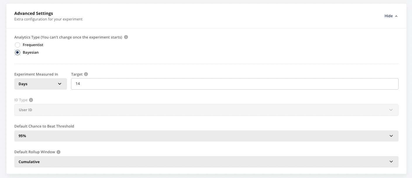
To switch an experiment to Bayesian mode, set Analytics Type to Bayesian under Advanced Settings on the experiment Setup tab. You can't change the analytics type after the experiment starts.
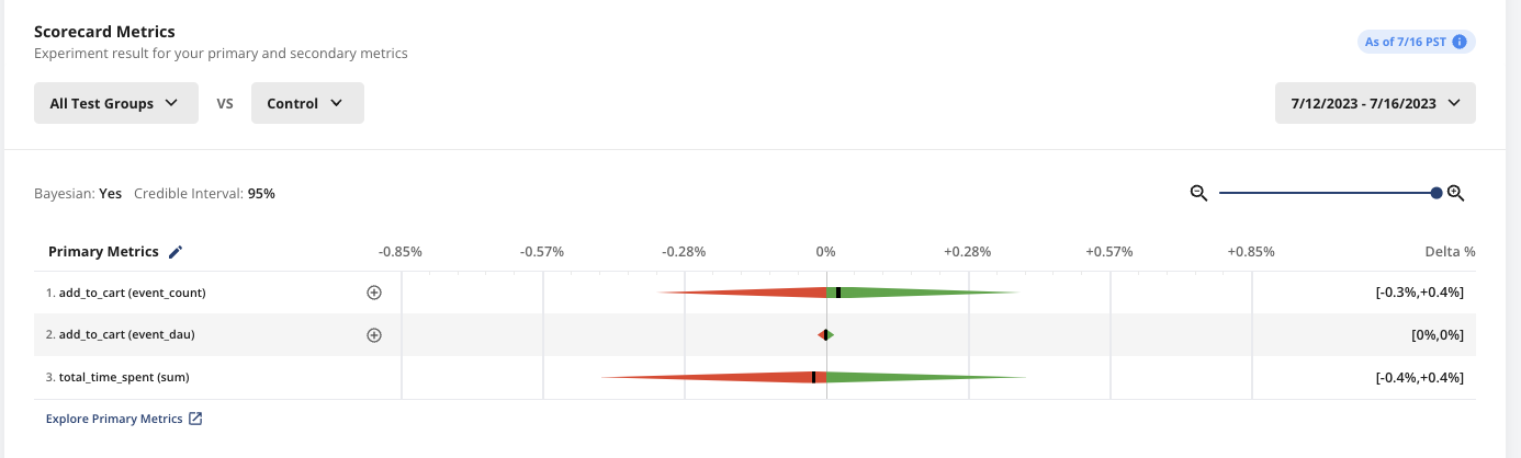
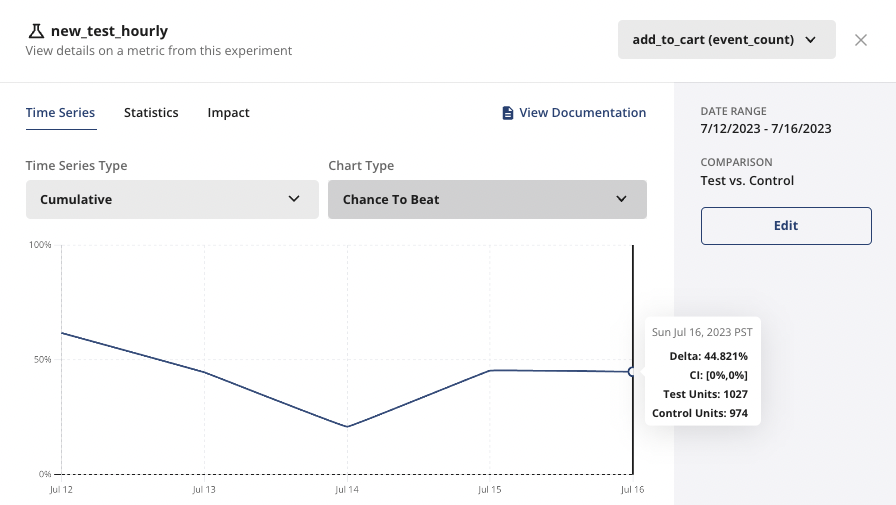
Pulse scorecard results and deep-dive analysis both reflect Bayesian statistics.
Informative priors
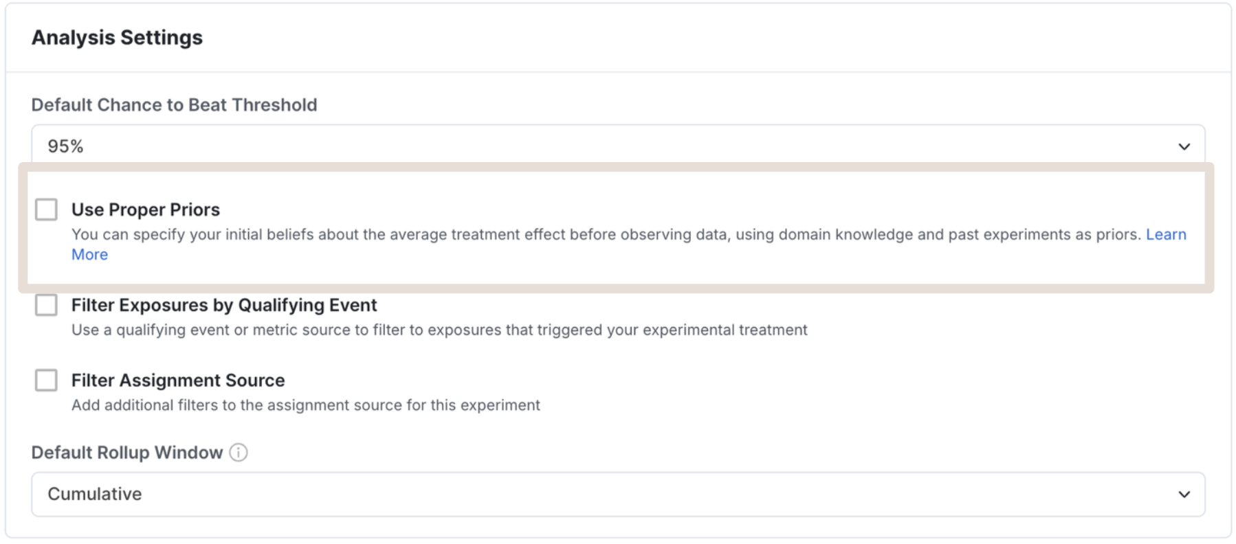
In Bayesian mode, you can set a prior belief on the relative average treatment effect. Statsig combines the prior distribution with the observed data and displays the prior-adjusted results. To turn on priors, select Use informative priors.
Deriving a prior from historical data
When you use informative priors, make sure your organization understands how the prior influences the experiment results, and base the prior on domain knowledge. Two common patterns:
- Use the of past experiments with a similar setup and population as the prior mean, and the standard deviation of those effects, or a multiple of it, as the prior standard error.
- Use the of past experiments as the prior standard error.
How Statsig computes the posterior
Denote as the prior distribution, where is the average treatment effect and is the standard error. Denote as the observed distribution.
Statsig calculates the posterior distribution as:
If you don't specify a prior, Statsig uses as the prior distribution .
Bayesian statistics glossary
Bayesian A/B tests use different terminology from the frequentist framework.
| Term | Definition |
|---|---|
| Credible interval | The interval that contains the true parameter at the given probability. |
| Chance to beat | The probability that the test group is better than control. |
| Expected loss | The average potential risk if you ship the test variant. |
Was this helpful?